Heat Stress Overlay tutorial: Difference between revisions
mNo edit summary |
mNo edit summary |
||
| Line 77: | Line 77: | ||
In addition, multiple times on a single day, and even multiple days, can be configured. When more than one moment in time is configured, the [[Heat Overlay]] will automatically calculate multiple [[timeframe]]s, each timeframe representing one discrete moment in time. | In addition, multiple times on a single day, and even multiple days, can be configured. When more than one moment in time is configured, the [[Heat Overlay]] will automatically calculate multiple [[timeframe]]s, each timeframe representing one discrete moment in time. | ||
{{page break}} | |||
Click on "Edit" to change the configured date/time. | Click on "Edit" to change the configured date/time. | ||
[[File:heat-options-2-edit.jpg|350px|frame|center|Click on "edit" to change the date and time(s).]] | [[File:heat-options-2-edit.jpg|350px|frame|center|Click on "edit" to change the date and time(s).]] | ||
The displayed hours are for the local timezone. | The displayed hours are for the local timezone. | ||
Revision as of 12:52, 22 October 2024
Prerequisites
The following prerequisites should be met before starting this tutorial:
- This tutorial relies on base knowledge about the editor interface and the creation of Overlays. If you have not yet followed the tutorials related to those subjects please do so first.
- This tutorial can be followed with any project of any arbitrary location in the Netherlands.
Preparations
Take the following steps as preparation for following this tutorial:
- Start your Project. This can be a pre-existing Project, or a newly created Project.
- The Project used should have a buffer of around 1km around the actual area of interest, so that the Heat Overlay calculation can account for broader spatial effects properly. A smaller project can be used, but will result in edge effects.
Introduction to the Heat Stress Overlay
The Heat Overlay allows users to visualize a generated Physiological Equivalent Temperature (PET) Overlay, along with other intermediate overlay results. The Heat Overlay can be configured using the Wizard.
Theory and background
The Heat Overlay's DPRA calculation mode is based on the DPRA Heat stress report of the RIVM. For more information on the origin of the underlying methods of calculations, please refer to this report.
The DPRA calculation method has been established by the dutch National Institute for Public Health and the Environment (RIVM). This approach has been created to calculate the physiological equivalent temperatures in an urban environment, based on both environmental weather conditions (such as ambient heat, radiance of heat from the sky, humidity, etc) as well as the effects of the built environments (such as shadows, vegetation, wind braking, etc).
The method makes use of weather measurements, such as those made available by the dutch Royal Netherlands Meteorological Institute (KNMI). Using weather data of specific representative days and/or moments allows for practical comparisons and verifications between the calculation method and the actual situation. The calculation method has been experimentally benchmarked by the RIVM by taking appropriate temperature measurements in the city of Wageningen on a significantly hot day (august 2nd, 2013), and veryfing the results of the calculation gave similar heat results geographically as the measurements indicated. The implementation in the Tygron Platform has been similarly benchmarked against these published results.
In addition, by using information of past days the weather conditions of which are expected to become more common in the future, it is very possible to make predictions about how heat-resiliant an urban environment will be in years or decades to come.
Adding a Heat Overlay
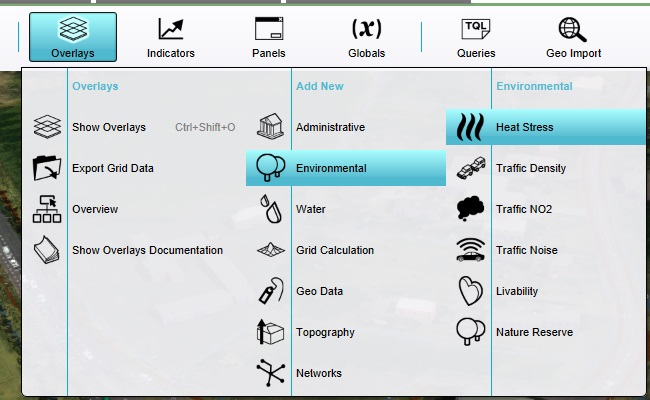
Add a Heat Overlay.
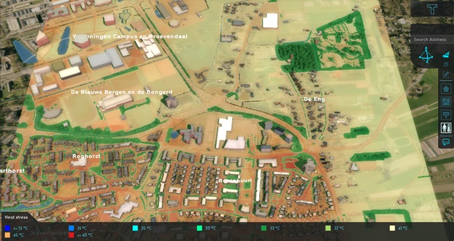
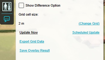
If the Heat Overlay does not immediately show results, click on "update now" in the right panel.
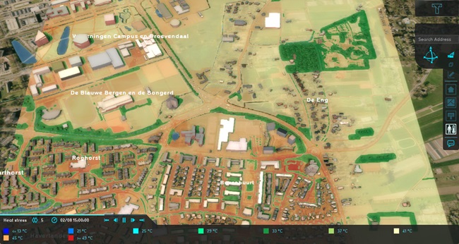
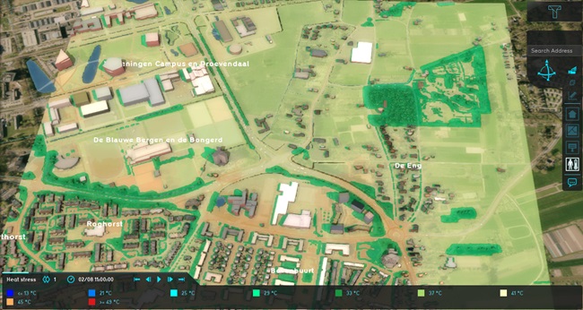
The Heat Overlay will show results, based on a default date and time, and its weather measurements. These defaults are based on the benchmark the RIVM has run, i.e. august 2nd, 2013, with weather station measurements from the Wageningen environment.
The default result of the Heat Overlay will be the PET, or Physiological Equivalent Temperature. This is how a given situation of temperature is experienced by an average adult human.
Options for the Heat calculation
To become more familiar with the options the Heat Overlay provides, the configuration wizard can be stepped through and all the options inspected.
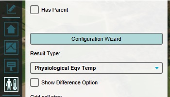
With the Heat Overlay selected in the editor, click on "Configuration Wizard" in the right panel.
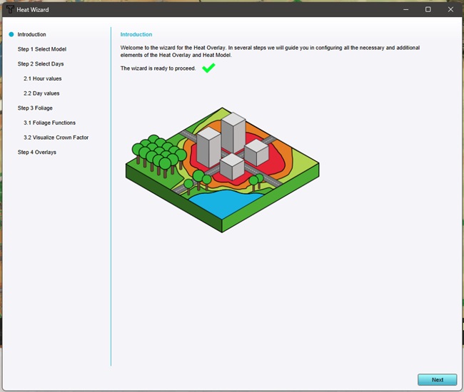
This will open the configuration wizard.
Click on "Next" to continue to the first step of the configuration wizard.
Heat model
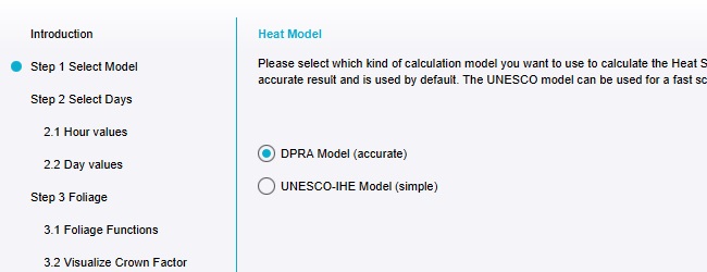
In the first step of the wizard, the applicable heat calculation model can be selected.
The DPRA model is the current and more accurate model. The UNESCO model is included for backwards compatibility reasions, but is no longer current or recommended for use.
Note that this tutorial is specifically for the DPRA model, disregarding the UNESCO model.
Ensure the DPRA model is selected.
Continue to the next step.
Days and hours
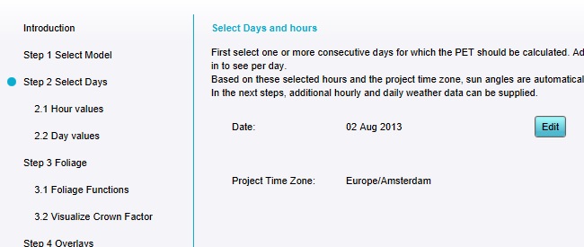
Next, the day and time for the calculation can be configured.
Based on the day, time, and the geographical location of the Project, the orientation and movement of the sun is automatically calculated.
In addition, multiple times on a single day, and even multiple days, can be configured. When more than one moment in time is configured, the Heat Overlay will automatically calculate multiple timeframes, each timeframe representing one discrete moment in time.
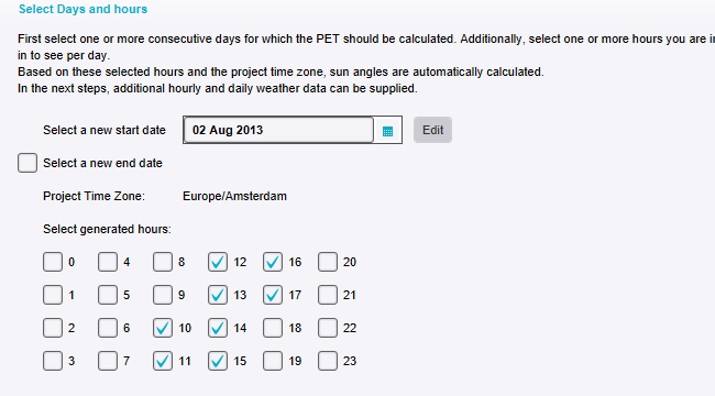
Click on "Edit" to change the configured date/time.
The displayed hours are for the local timezone.
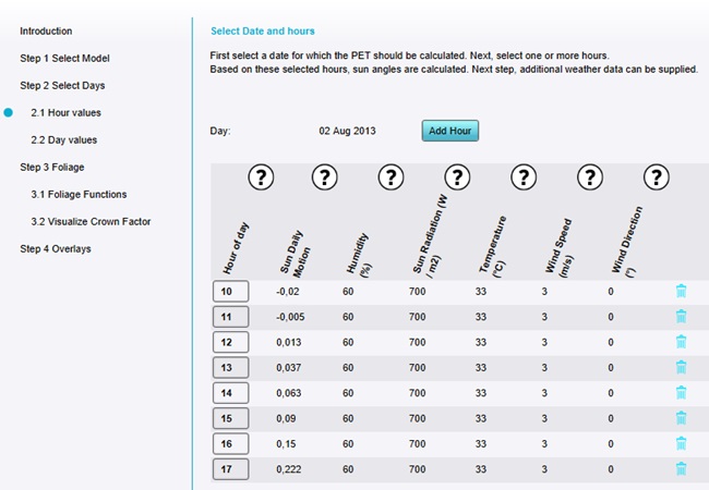
Ensure the following hours are selected:
- 10
- 11
- 12
- 13
- 14
- 15
- 16
- 17
Continue to the next step.
For every hour, specific weather measurement data can be configured to represent the changing weather conditions over the day.
For now, only take note of the kinds of data which can be configured in this step.
Continue to the next step.
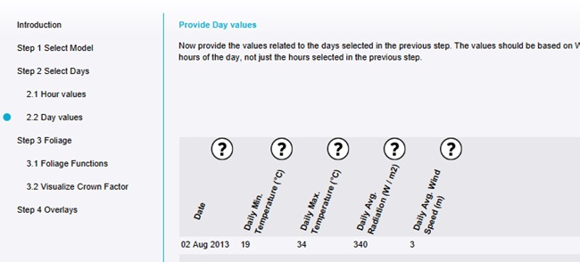
Besides a configuration per hour, averaged information for each given day is also required.
As with the hour information, for now only take note of the kinds of data which can be configured in this step.
Continue to the next step.
Foliage
One of the most impactful ways heat stress can be affected is through the use of foliage to create shade in an urban environment.
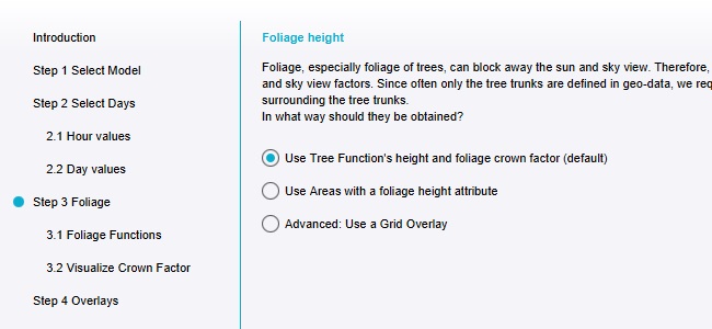
The Heat Overlay specifically requires foliage information to properly compute the height and location of shade. If no data specifically related to foliage is available in the Project, foliage data can be derived from Buildings such as trees.
- Functions
- When deriving foliage from tree Functions, foliage is determined based on the tree's height, and a foliage crown factor, which is the ratio between the tree's height and the width of the crown. The height of the foliage near the centre of the tree will be higher than the height of the foliage near the edges of the crown. This is the default mode.
- The benefit of this approach is that it can be derived from data which is already almost always available in a Project. In addition, the calculation will also be immediately responsive to changes in the Buildings data, for example when testing Measures or other Future Designs. It has the downside that the computed foliage has a consistent and assumedly circular shape.
- Areas
- If there is foliage information available in the Project in the form of Areas, the Heat Overlay can be configured to look for a specific Attribute attached to these Areas. If such an Attribute is found, then the model will use the polygon of the Area(s) and the value in the Attribute as direct input for foliage information.
- The benefit of this approach is that more detailed shapes for foliage can be loaded in. The downsides are that the foliage will be considered of a uniform height per polygon, and that changes in the urban environment (such as the creation or removal of trees) are not translated into a new foliage situation.
- Grids
- Finally, and most ideally, foliage information can be provided as a grid. Grids provide the most detail, in that they can represent both varying foliage heights as well as varying foliage shapes.
- The benefits of using grids include the fact that they are easily managed as a single dataset, can be loaded in without colliding with other data, can be manipulated by the Tygron Platform's Combo Overlays when desired, all while offering a highest level of detail. The downsides are that like Areas, the existence of foliage is not directly affected by changes in the urban environment such as the creation or removal of trees.
As there is no guaranteed additional dataset available to indicate foliage information, ensure the foliage method is set to "Tree Function".
Continue to the next step.
Foliage configuration
Depending on the selected mode for foliage determination, one or more additional minor steps are available to configure this mode.
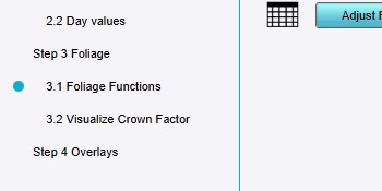
Because the model is now set to use the default foliage determination based on Functions, some options to change those Function Values are available, as well as options to gain insight into the presence of those values, are available. These options can be skipped.
Continue to the next major step.
Output overlays
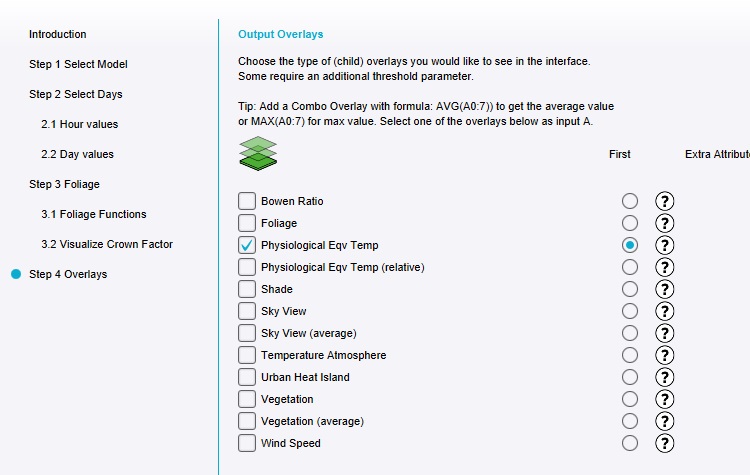
The last step for the proper configuration of the Heat Overlay is selecting the desired outputs.
The calculation of the Heat Overlay takes place over multiple steps, parsing and combining different elements of geographical and non-geographical data to compute inputs for the next steps. For example, the Urban Heat Island is calculated based on features in the built environment, which in turn affects the heat retention and radiation.
The final result of the calculation is the Physiological Equivalent Temperature. The other options are intermediate results which may provide insight into the major component effects for the calculated heat stress, or be relevant in and of themselves such as the result of shade.
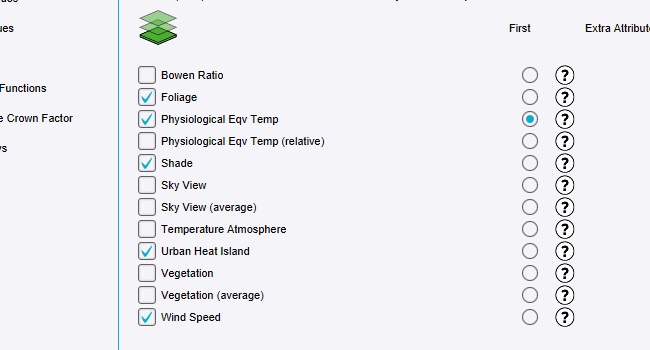
Ensure the following outputs are selected:
- Physiological Equivalent Temperature
- The end result of the heat stress calculation. This is how a given situation of temperature is experienced by an average adult human.
- Foliage
- The presence of foliage in the project area, as interpreted by the Heat Overlay, expressed as height of the foliage above the surface of the terrain.
- Shade
- The presence of shade in the project area, calculated based on the orientation of the sun and the Digital surface model.
- Urban Heat Island
- The calculated urban heat island, which represents the capacity for heat retention of the built environment.
- Wind Speed
- The calculated wind speeds, based on the wind speed provided as part of the weather data, and the presence of Buildings which can limit the free flow of air.
Click on "Finish" to close the wizard.
View calculated results
With the Heat Overlay selected in the editor, click on "update now" in the right panel to recalculate the results. This will include both the end result of Physiological Equivalent Temperature, and the child Overlays with intermediate results previously selected.
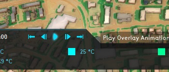
When the calculation has completed, in the Viewer interface, click on the "play" button in the legend of the Heat Overlay.
This will show a progression of results, one snapshot for each moment in time as selected in the configuration wizard.
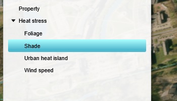
In the left panel, open the list of child Overlays of the Heat Overlay.
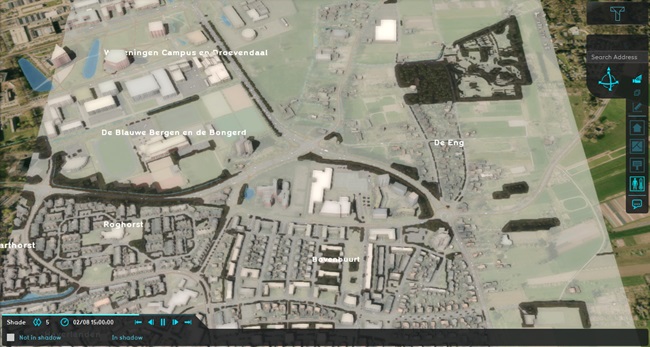
Select the Shade result.
Again, click on the "play button".
Notice how the calculated shades move across the built environment.
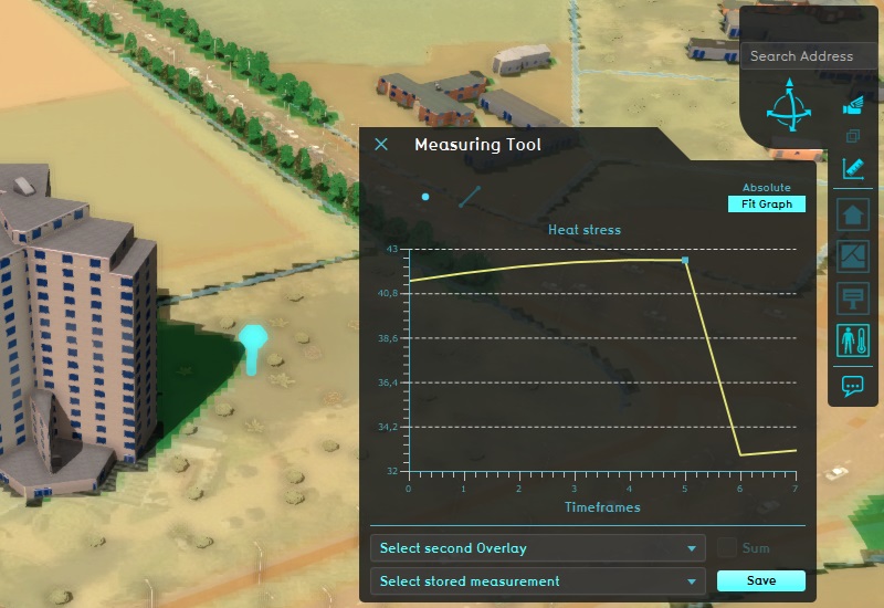
Switch back to the main Heat Overlay. Then, on the right-hand side of the Viewer interface, click on the "Measurement tool" icon.
Click in any location in the 3D world to see how the temperature in that location progresses over time. Click on "Fit Graph" to scale the results for improved legibility.
Configuring weather data
The changes in heat stress over the day are, with the current configuration, entirely driven by the changes of the effects of the sun. This is because no detailed weather data has been added yet.
Configuring the Heat Overlay's weather parameters is important to create a more realistic and detailed result of calculated heat effects.
Note that these steps are mainly described in the context of Projects location in the Netherlands. For locations outside of the Netherlands, the default location of Wageningen could be used, but this should be done with care as that weather effect may not be appropriate for another Project's location.
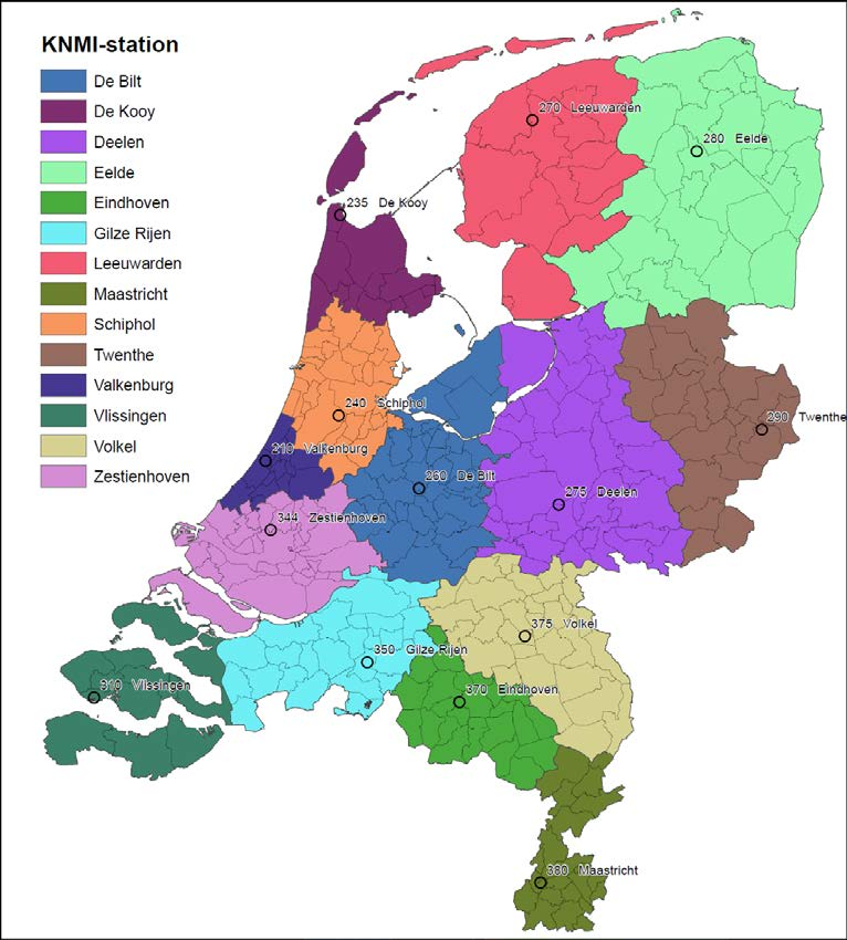
To set up this configuration, the appropriate weather station should be determined. Consult the following map to determine which weather station is most appropriate for the Project's location, and take note of the station's ID number.
A more detailed list of weather station recommendations can be found on the appropriate support wiki page:
https://support.tygron.com/wiki/Dutch_weather_stations
Next, the data of that particular weather station can be downloaded directly from the site of the KNMI. The downloads can be found here:
https://www.knmi.nl/nederland-nu/klimatologie/uurgegevens
Find the weather station previously determined to be most appropriate for the Project's location, either by name or by ID number.
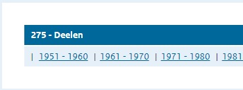
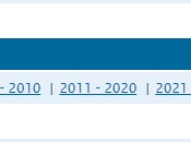
Next, select the desired decade. For example, the climate data for the 2nd of august 2013 can be found in the 2011-2020 decade.
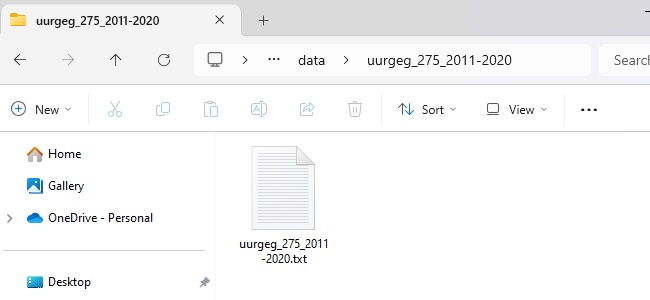
This will start the download of a zip file.
Once the download has completed, unpack the zipfile. This will allow access to a single txt file, which contains data structured as comma-separated values.
This csv file can be opened in Microsoft Excel.
Start Microsoft Excel.
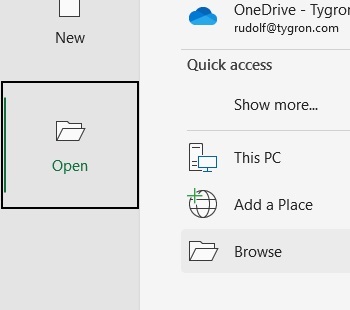
In the Welcome screen, opt to open a file, and select "browse". This will open the file selection screen.
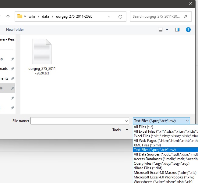
At the bottom-right of the file selection screen, set the file type to "text files", which include ".csv" files.
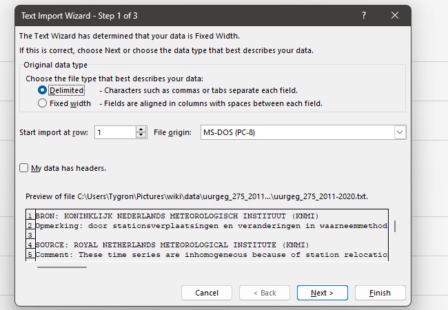
Select the .txt file downloaded, and opt to open it. This will open the "text import wizard".
For the file type, select "Delimited", and click on next.
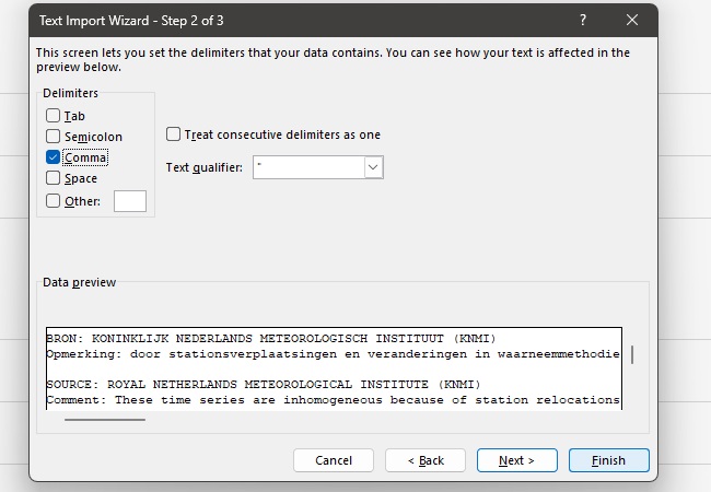
For the separator, select "Comma", and click on "Complete" to finish the wizard.
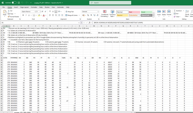
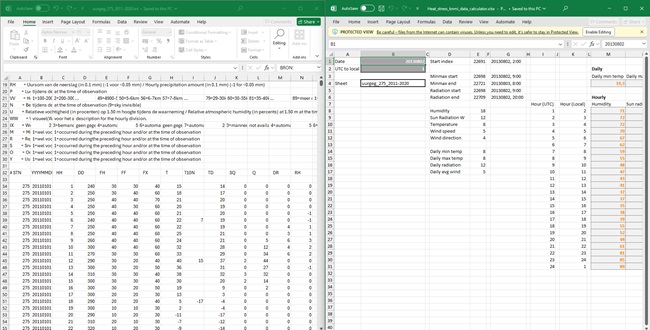
The KNMI weather data is now opened as a functional Excel workbook.
Note that the following step of parsing exact data from the workbook is described in reliance of an additional Excel file as assistive tool. Parsing the data can also be done manually, but this is a more involved process.
Download and open the Heat Stress KNMI data calculator Excel File.
https://support.tygron.com/wiki/File:Heat_stress_knmi_data_calculator.xlsx
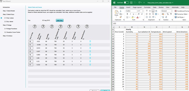
You should now have one Excel instance open with the downloaded data, and a second Excel instance with the calculator tool.
Ensure editing is activated for both files.
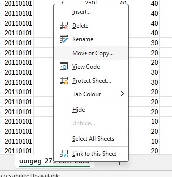
In the Excel instance with the downloaded data, right-click on the data's workbook tab, and select "Move or copy..."
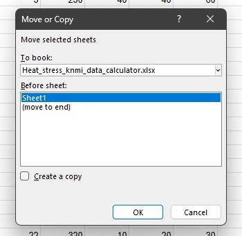
Opt to move or copy the data to the other Excel instance, with the calculator tool.
When the operation has completed, in the Excel instance with the calculator tool, switch to the "Calculator" tab.
In cell B4 (preceded by "Sheet"), change the name of the target sheet to the dataset now added. This will direct the calculator to consult the data you downloaded and added.
In cell B1, select the desired date.
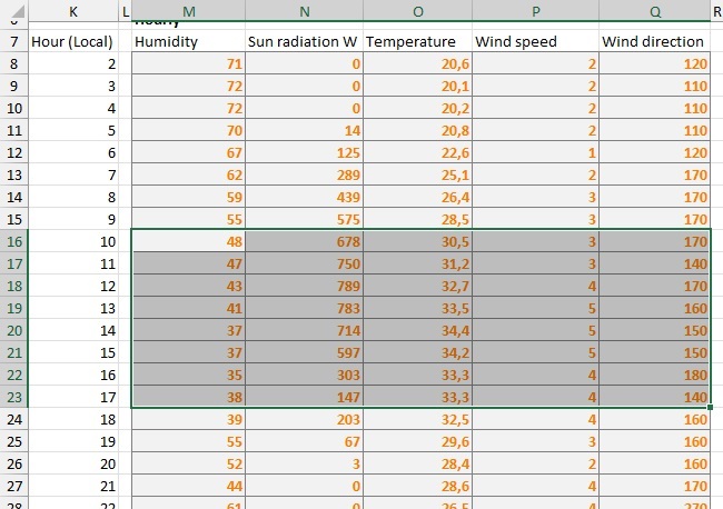
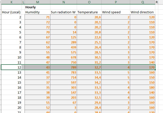
Columns M through Q now show the appropriate values which can be entered into the Heat Overlay's configuration wizard. For each hour-of-the-day as listed in the configuration wizard, the appropriate hour-of-the-day can be found in column K.
For example, the row of values where column K has the hour "12" listed, should be entered in the Heat Overlay's configuration wizard for the hour-of-day 12.
In the Tygron Client, reopen the Heat Overlay's configuration wizard and continue to the step for date and time selection.
Ensure the appropriate date for the Project is set.
Continue to the step for hour values.
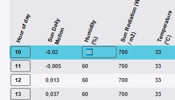
Starting with "Humidity", double-click on the first value listed.
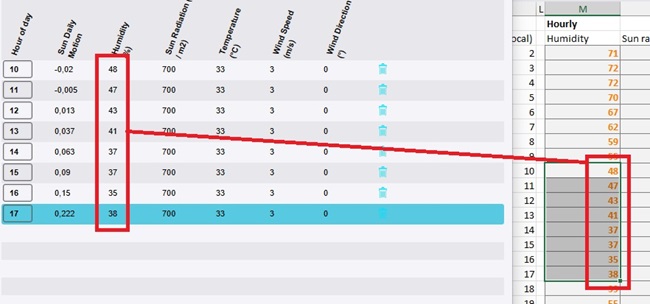
Enter the value listed for that (local) hour in the calculator tool. Then press enter.
Repeat this for all humidity values for the applicable (local) hours.
Repeat this for the other hourly weather values as well.
In the configuration wizard, continue to the next step for the daily values.
The daily values are calculated in row 4, in columns M through P. Enter the values listed there in the configuration wizard as well.
After entering all the values, close the configuration wizard. Then, in the right panel, click on "update now".
The results are now different, most likely more nuanced, and more accurate for the indicated day and location.
Final assignments
- Find a location which is in shade only part of the day. Use the measurement tool to see the values of shade over the day and compare it to the values of heat over the day.
- For the Heat Overlay, activate the "Show Difference" option. Repeat this for the child Overlays. Next, add trees to the Project area as an Action or a Measure.
- Investigate the Heat Overlay, with emphasis on the difference view of the Overlay. Do you see the spatial effects of the taken Action?
- Investigate the Shade result, with emphasis on the difference view of the Overlay. Do you see a (partial) correlation between the changes in shading and heat?
- Investigate the wind speed result, with emphasis on the difference view of the Overlay. Do you see a (partial) correlation between the changes in wind speed and heat?
Final notes
Although not part of the general explanation provided in this tutorial, the following notes are important to keep in mind:
- More information on the theory behind the DPRA Heat Stress calculation method can be found in the RIVM's DPRA Heat Stress Report.
- More information on the theory and implementation of the model in the Tygron Platform is available in the documentation regarding the Heat Module theory implementation.
- More information on the potential outputs of the heat stress calculation is available in the documentation regarding the result types of the Heat Overlay.
Tutorial completed
Congratulations. You have now completed this tutorial. In it, you have learned how to add, interpret, and configure the Heat Overlay. The next tutorial in this series is Trees and foliage, which will provide more knowledge about managing and updating foliage data, with an emphasis of use with the Heat Overlay.
