Testbed tutorial
Prerequisites
The following prerequisites should be met before starting this tutorial:
- This tutorial relies on base knowledge about the editor interface. If you have not yet followed the tutorials related to those subjects please do so first.
- This tutorial can be followed in an empty project area.
- Knowledge of the functioning of the water module is recommended, but not required.
Preparations
Take the following steps as preparation for following this tutorial:
- Create a new, empty project, sized to 500m by 500m. Ensure the unit system is set to "International". Also ensure it's an empty project area, not based on a real world location.
Introduction to testbeds
A testbed is a controlled setup, in which there are as few variables as possible which could influence a given situation.
In the Tygron Platform, whenever you create a project based on real-world data, the project is populated with a wide range of data. Virtually every project area contains numerous constructions, height differentials, and terrain types. If any calculation takes place, especially spatial calculations, all that data can serve as input. That makes it a lot more difficult to see exactly how a specific element factors into a specific result, or where the difference between an expected and actual result comes from.
Testbeds can serve the following purposes:
- Quick investigations into how a specific functionality works
- Overview demonstrations of multiple functionalities
- Forming a baseline for consistency testing
- Testing for (and demonstrations of) bugs or other issues
For this reason, what characterizes a testbed most is the absence of data. Anything that is not requires for a specific case is left out, or at least left in a uniform, invariable state.
Starting point
For each testbed, the starting point is the empty project.
An empty project contains the following data:
- There is a uniform height map, with the height of the terrain set to 1m relative to datum.
- The surface of the terrain is of the "Open Land" type. The underground terrain is of the "Unknown" type.
- There is only a single municipal stakeholder, as a stakeholder to select for an editing user. The entirety of the 3D world is owned by that stakeholder.
- There are 4 neighborhoods (north-west, north-east, south-west, south-east), or if the project area is small, 1 single neighborhood.
- There is no zoning plan.
- There are no construction.
- The upper-left spatial coordinates of the project area are set to 0 degrees latitude and longitude.
Quick functionality testing
Testbeds can be used to test specific implementation questions. The question you're going to investigate is how the average overlay calculation functions in cases where the calculation takes place near the edge of the project area.
The average overlay functions by, for any given grid cell, looking at the surrounding grid cells, calculating the average value of the cells found. In most locations in a project area this calculation is very straightforward. However, if any of the cells looked at would fall outside the project area, any number of behaviors could be reasonable. For example: the cells outside the project area could be assumed to have a certain default value, or the cells could be disregarded for the calculations. You will configure the testbed to reveal how the average overlay deals with cells outside the project area.
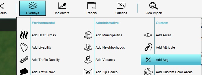
Start by adding the overlay we're going to test. Add an average overlay to the project.
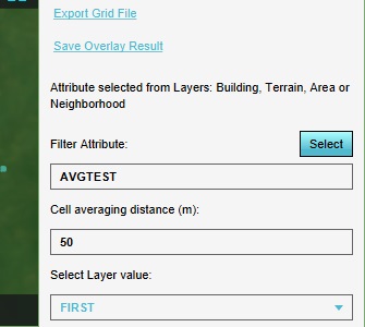
Prepare the overlay in such a way that it will calculate the spatial average of a user-defined attribute. As Filter Attribute, enter "AVGTEST". Also set the Cell averaging distance to 50m. This will ensure that multiple entities can be drawn in the map and be spatially calculated, without necessarily affecting each other's outcomes.
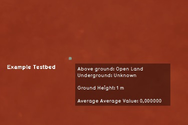
With this configuration, the calculation will result in a value of 0 in every location.
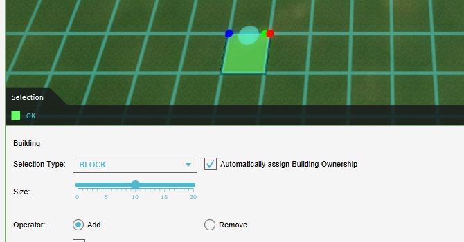
Now add a construction to the project, and place it more or less in the center of the project. Make sure you use the block-based brush, and draw in exactly 1 block (10m by 10m, for a total of 100m²).
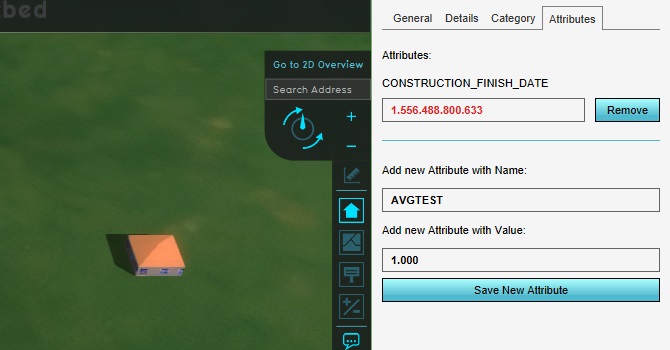
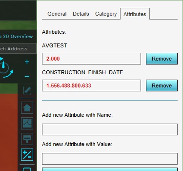
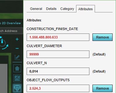
Add an AVGTEST attribute to the construction, with a value of 1000.
Switch back to the average overlay in the editor, and select "Update Now" to recalculate the content
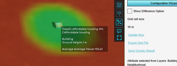
Now, if you open the average overlay, you will see the construction is the center of a large area where the average value of AVGTEST is higher than in all other locations in the project area.
This setup creates a first look into how the average overlay functions. In the exact location of the construction, and its direct surroundings, the average value of AVGTEST is around 130. It tapers of at a distance of about 50 meters.
Note that you may see a value lower than 130, based on the exact location you have placed the construction. This is due to the construction's alignment on the calculation grid. This is expected, and does not affect the principles explained next. Take note of the value you see in your project, and continue.
We can now add another construction to the project, again with an AVGTEST attribute set to a value of 1000, and place that construction in the corner of the project area. Again, making sure that the construction is exactly 1 block of 10m by 10m, for a total of 100m².
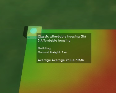
Recalculating the overlay and looking at the average value at the location of the new construction gives an average value of 180.
The fact that the calculated value in the corner is higher indicates that the cells outside the project area don't have an assumed value of 0 or lower.
Increase the AVGTEST attribute value of both constructions to 2000, and check again what average values are calculated in the locations of the constructions.
Now when you look at the calculated average value at the location of the construction, you will see that after doubling the attribute of the construction, the calculated value has doubled as well (give or take a rounding).
We can now put the following facts together:
- An average is a value calculated as follows: The sum of all values found in the calculation area, divided by the calculation area.
- The calculated average scales linearly with the value of the object we place. This means that the cells outside the project area do not have a positive or negative value. If they did, the impact of raising or lowering the attribute value would have been more or less impactful.
- An object at the edge of the project area has a greater impact on the calculated spatial average than a construction in the middle of the project area. This means that either the sum of all values increases as we get closer to the edge, or the surface area we divide by decreases.
We can determine that because the summed value does not change, the surface area used in the calculation must decrease in order to see the higher result. Thus our conclusion is that potential cells outside the project area are not used in the calculation of a spatial average.
Considerations
Note that based on the conclusion we have drawn, you may be tempted to expect the calculated values to match more neatly. Specifically, if the construction in the middle of the map has a full circle around it in which to perform its calculation, the construction in the edge of the map must have a quarter of the area of similar circle, thus the values should differ by a factor of 4. However, due to the layout of the constructions on the grid this is not the case.
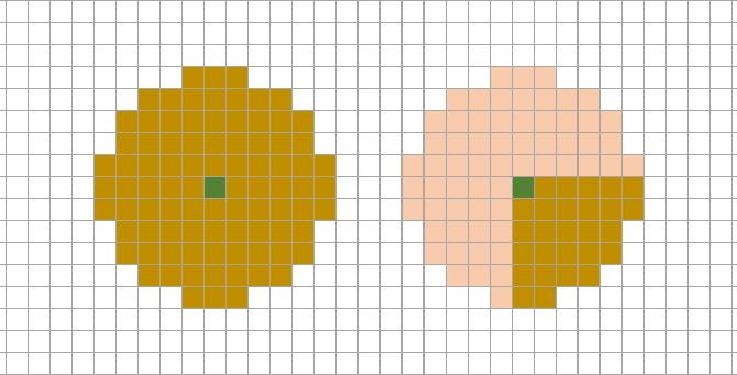
Also note that based on the exact size, placement, and rounding of values and polygons, it may be difficult to derive the outcomes seen from the base values without greater insight into the exact interpretations the Tygron Platform makes. This is to be expected, and the approach used here functions regardless of those exact calculations.
Assignments
These assignments are designed to demonstrate further means of experimentation.
- Knowing the radius of the spatial calculation is 50m, place a construction with the same attribute and value as close to the edge of the map as possible without the calculated average value differing from the construction in the middle of the project area.
- Change the average attribute of the constructions back to 1000, and instead expand both constructions with another block of 10m by 10m. Both constructions should be exactly twice as large as they were.
- Knowing the grid cell size is exactly 10m by 10m, find an explanation for the fact that both 'sides' of the construction in the middle of the map have the same calculated average, but the sides of the construction in the corner of the map do not.
Model functionality demonstration
Testbeds can also be used to give an overview of multiple aspects of a model or functionality. These testbeds can take on the form of a single project with multiple isolated setups, or of one larger interconnected system. The question you're going to investigate now is how the water overlay deals with height differences.
"Height" is a broad concept, which means there is no singular detail to highlight. Instead, the proper approach is to see how height affects a basic setup, and then expand from that basic setup into slightly more complex configurations. The intent is to create an effective sense of how height is taken into account.
Either create a new empty project with the same specifications as in the prerequisites, or clean up the project configured during the last assignment by removing the added overlay and construction. Either way, make sure you start with an empty project area again.
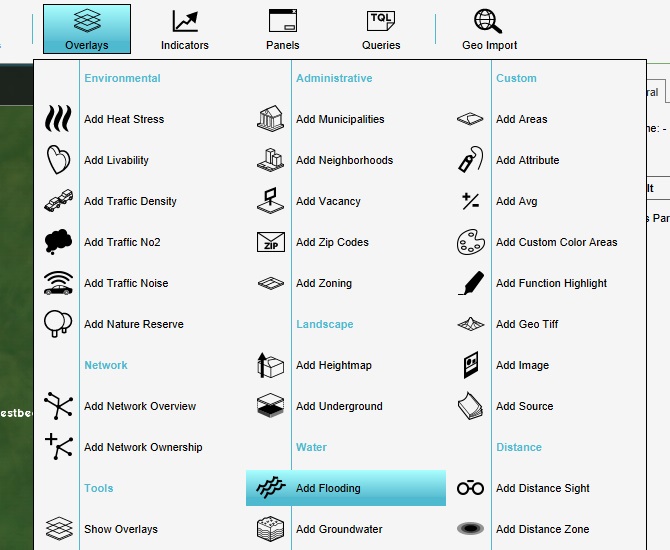
Start by adding the overlay we are going to test. Add a flooding overlay to the project.
Direct flow
The most basic setup to create is one where water directly flows from a higher location to a lower location.
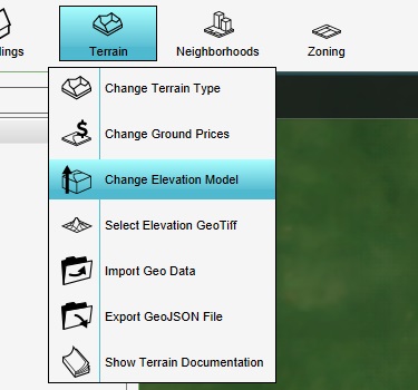
Open the terrain's change elevation tool. You will use this to change the height of the terrain to create the necessary setup.
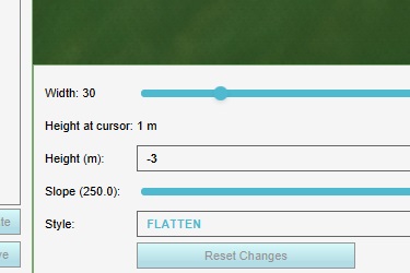
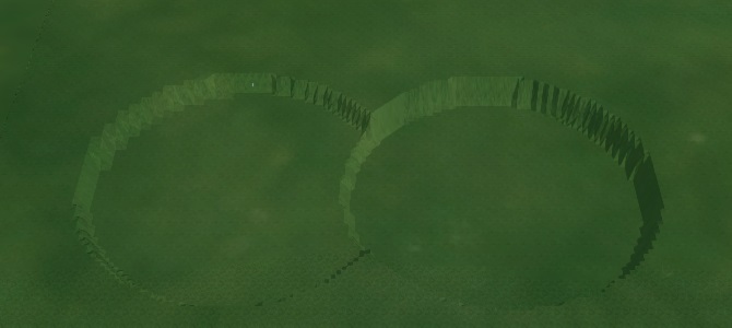
This will open the terrain elevation brush panel in the bottom of the editor. For simple setup, we will create 2 indentations in the terrain, directly attached to one another and one deeper than the other.
Configure the brush as follows:
- Width: 30 (meter)
- Height: -3 (meter)
- Slope': 250
- Style: Flatten
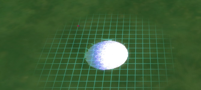
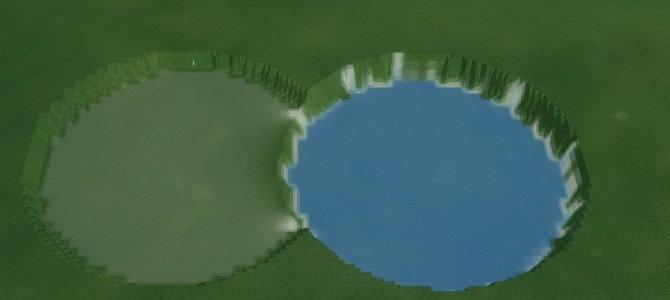
This will create a hole, with a radius of 30 meters, and a depth of 4 meters. (the project area's default height is 1 meter above datum, and the specified setting will place the bottom of the hole at 3 meters below datum, so the total depth will be 4 meters)
In the 3D world, click anywhere in the project area, such that the entire hole is inside the project area. (If you are having trouble determining where the edge of your project area is, try placing a construction in the corner of the project first, as a navigational aid. Adding a construction will not affect the model we are setting up.)
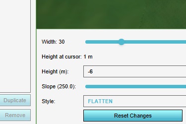
Next, change the "height" setting of the brush to -6.
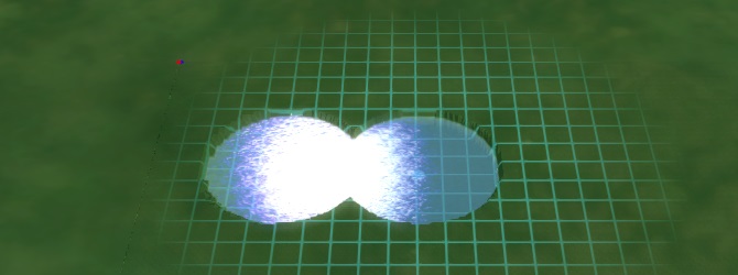
Now place another hole in the 3D world, such that the first hole and the second hole are connected.
Finally, click "Apply Changes" to complete the adjustment of the terrain height.
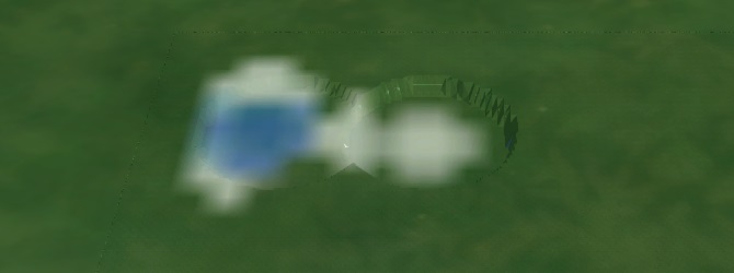
Now that the heightmap is changed, you will be able to properly see the created holes.
Now we have a basic height difference. The reason for creating 2 pits instead of 1, is to make sure that water which is used in this test remains in this test, and does not flow of into other places. If water is allowed to flow away, then at least its not possible to account for all the water in the end result, and at worst the water may affect other tests.
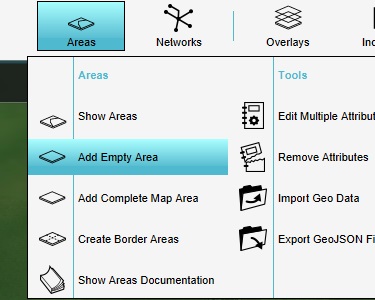
Add an area to the project. Set the name of the area to "Inundation 1".
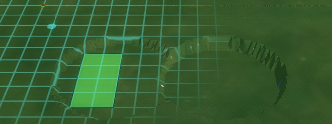
Draw the area in the project area. Specifically, make sure it sits inside the higher of the 2 hole, with no edges on the normal surface.
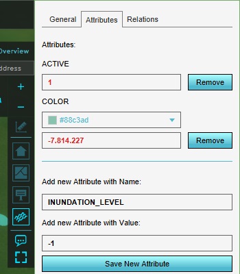
Add the attribute "INUNDATION_LEVEL" to the area, with a value of "-1". In the context of the flooding overlay, this means this area has a column of water up to the height of -1 meter relative to datum. The bottom of the hole being at -3 meters relative to datum, the column of water will be 2 meters high, but still 2 meters below the surface of the rest of the terrain.
Looking at the current result of the flooding overlay's calculation, it's clear that the results are rather crude.
This is due to 2 default configurations for the flooding overlay, namely the grid cell size affecting how accurate the results are, and the result type which affects what the results are.
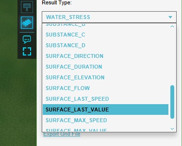
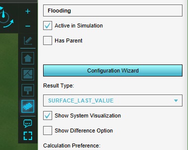
Currently, the result type is WATER_STRESS, which shows the highest amounts of water which existed in a cell at any point during the overlay's calculation. Set the result type to SURFACE_LAST_VALUE, which shows the exact amount of water present in any cell at any given point in the calculation.
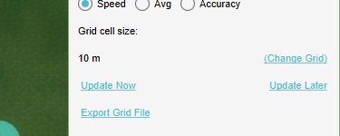
Next, select "Change Grid".
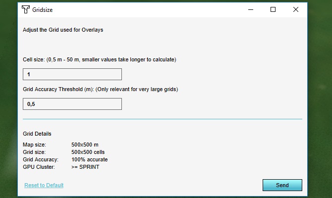
Change the grid cell size settings as follows:
- Cell size: 1 meter
- Grid accuracy threshold: 0.5 meter
This will greatly increase the accuracy of the calculation. Due to the simplicity of the model, the calculation times will still be extremely low.
Click "Send". After the overlay has recalculated, you will see the end result of the flooding calculation has changed.
Use the timeframe controls in the overlay's legend to switch to the first timeframe.
What you'll notice specifically is that the calculation's results is composed of 10 timeframes. Each of the timeframes represents a snapshot of the process of water flowing into the deeper hole. However, the water flows so quickly that even at the first timeframe most water has already flowed into the lower hole. This means the timescale of the simulation should be tweaked as well.
Select the overlay in the editor, and open the configuration wizard.
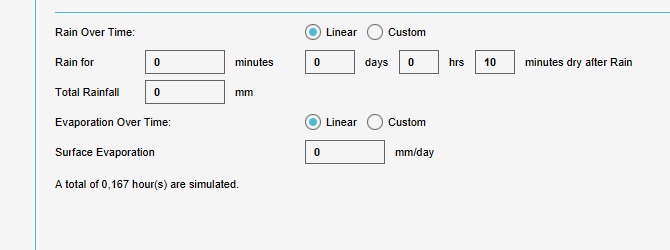
Click "Next" to continue to the weather configuration step. In this step, set the following configuration:
- Rain for 0 minutes
- Total rainfall 0 mm
- 0 days, 0 hours, 10 minutes dry after rain
- Surface evaporation of 0 mm/day
Close the configuration wizard, and click "Update Now" to force the overlay to recalculate.
Now using the timeframe controls, its possible to see how the water moves into the lower hole over time.
For a basic impression of the flow of water, this is sufficient.
Culvert flow
A slightly more complex setup is one where the 2 holes aren't directly connected to one another, but via a culvert set at a specific height.
Open the terrain elevation tool again. Configure the brush as follows:
- Width: 30 (meter)
- Height: -3 (meter)
- Slope': 250
- Style: Flatten
In the 3D world, pick a location for another setup, without it overlapping with the first setup. Click in the 3D world to create a new hole. Create another hole next to it, in such a way that there is still some room between them. Both holes should now be identical.
