|
|
| Line 1: |
Line 1: |
| In this tutorial we will configure a [[Rainfall_(Overlay)|rainfall overlay]]. After this tutorial, you will be able to configure a [[Rainfall_(Overlay)|rainfall overlay]] by making use of the [[Water_Overlay_Wizard|configuration wizard]] and have learnt what kind of data is used as input for the [[Water_Module_Theory|water module]].
| | __NOTOC__ |
| | {|class="wikitable" style="margin: auto; background-color:#ffffcc;" |
| | | [[Demo_San_Francisco_Project_FAQ_%26_More|Next page>>]] |
| | |} |
| | [[File:San_francisco.png|thumb|right|300px|Project of San Francisco in the {{software}}]] |
| | {{demo project summary |
| | | title=Demo San Francisco |
| | | demographic= you if you are interested in GIS, BIM, data analysis, 3D visualization, urban planning and architecture |
| | | showcases= a 3D city model |
| | | image= |
| | | description=The ''Demo San Francisco'' project is a working project which shows an area in the San Francisco financial district, created from, among others, [[SLPK|I3S Scene Layer data]] and [[Project_Sources|OSM]] data. The demo project contains an analysis on the sky visibility from street level and insight into land use and building type. In this demo we will explore the contents of the 3D model, the used data to generate the model and the maps on building type, sky view and land use. |
| | | tutorial= |
| | }} |
|
| |
|
| ==Getting Started== | | ==Explore the current situation== |
| # [//tygronsupport.freshdesk.com/support/tickets/new Contact Tygron Support] to request the Kockengen Tutorial project | | # Zoom and click around in the project to inspect the 3D model. |
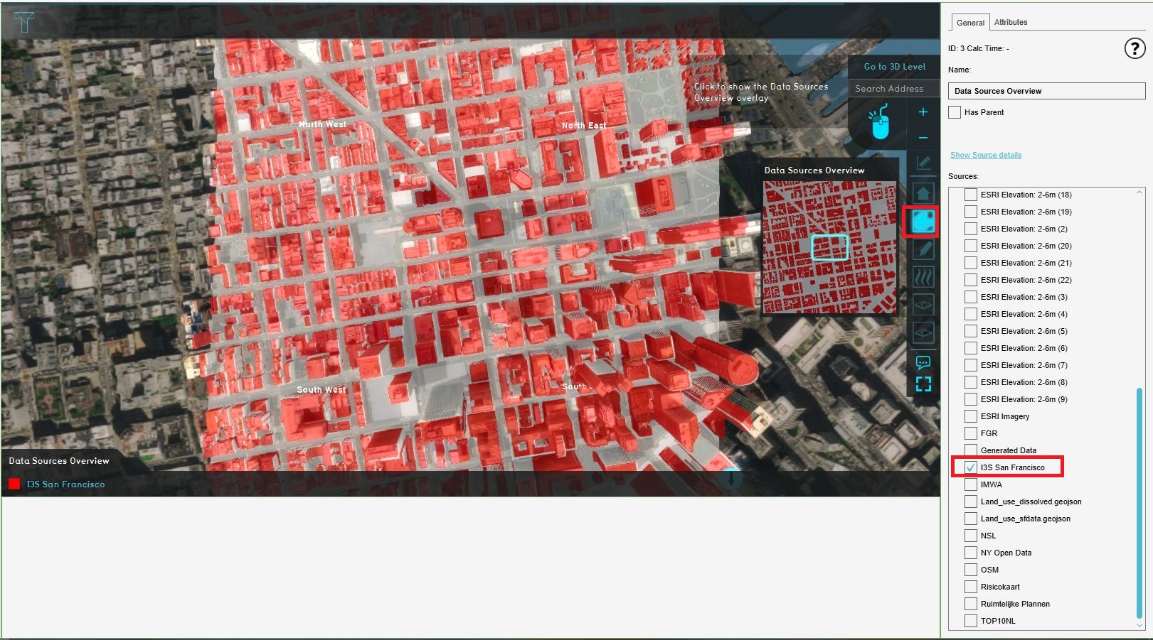
| # Open the {{software}}, logon with your user name and password and open the project ''Kockengen Tutorial'' | | # Click in the Current Situation tab on the Overlays button and click in the left panel on Data Sources Overview. This map, the [[Source_(Overlay)|Source overlay]], highlights the used datasets in a 3D model. Notice the I3S San Francisco dataset is checked in the right panel. Notice most of the buildings in the 3D model are highlighted. This means data from the I3S Scene Layer is used to create these buildings. The black ribbon on the right is the overlay bar. Here you will find several [[Overlays|Overlays]]. An overlay is a 2D map on top of the 3D world. Notice that the palette icon is highlighted. The Data Sources Overview corresponds with the palette icon. Therefore to show the Data Sources Overview, you can also click on the palette icon. |
| # Download and unpack the content of this zip-file on your desktop: [http://downloads.support.tygron.com/tutorials/kockengen_data.zip] | | [[File:Sources_i3s.JPG|150px|Notice that the I3S dataset is checked. The Data Sources Overview shows where the I3S data is used.]] |
| | # Uncheck the I3S San Francisco dataset in the right panel and check the [[Project_Sources|OSM]] dataset. Notice that again almost all buildings are highlighted. This accentuates the effect that the {{software}} uses multiple data sources to create the 3D model. Take a look at the [[Project_Sources|project sources]] page to see all the (open) data we use to generate a new project. |
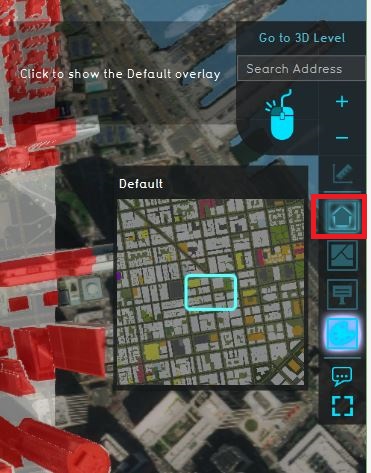
| | # [[File:City_overlay.JPG|right|150px|Click on the City overlay to go to the default view. ]]Click on the [[City_Overlay|City overlay]] in the overlay bar, depicted with the house icon to see the default 3D model without a map.{{clear}} |
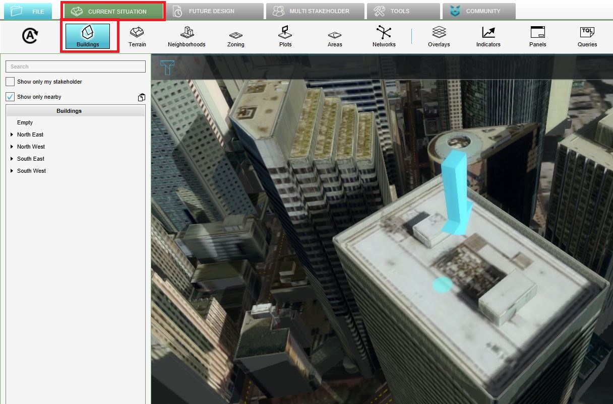
| | # [[File:Attributes_building.JPG|right|150px|The attributes of the building.]][[File:Select_building_project.JPG|right|150px|Click in the Current tab on the Buildings button and click on the building with the arrow.]]We are going to inspect one of the buildings in the model. Therefore click on the [[Current_Situation|Current situation tab]] on the [[Constructions|Buildings]] button and select the building that is referred to with the arrow icon. In the right panel, the attributes such as the name of the building and its [[Function|function]] are displayed. Notice that this building has the function office, which is known from the [[Project_Sources|OSM]] dataset.{{clear}} |
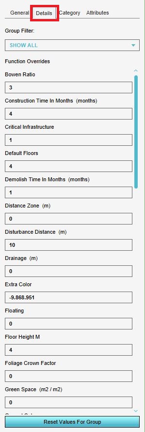
| | # Select the Details tab and scroll through the different attributes and values. These attributes are called [[Function_Value|function values]]. Notice that some attributes have values and some attributes have a value of 0. These values are used in our [[Calculation_Models#Calculation_Models|calculation models]]. |
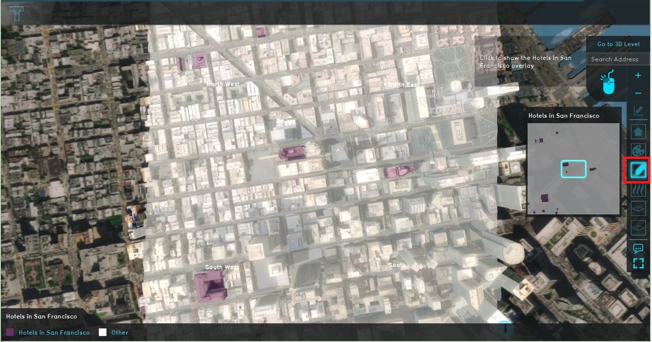
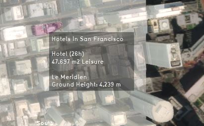
| | # Click again on the [[Constructions|Buildings]] button to close the menu on the right and click in the overlay bar on the [[Function_Highlight_(Overlay)|Function highlight overlay]] depicted with the pen icon. This overlay can highlight one or more functions in the 3D world. Notice from the legend this overlay shows the hotel [[Function|functions]]. |
| | # Zoom out a bit so that the whole 3D world is visible and click on the highlighted purple buildings. Notice that a hover panel pops up which also contains some information about the building. |
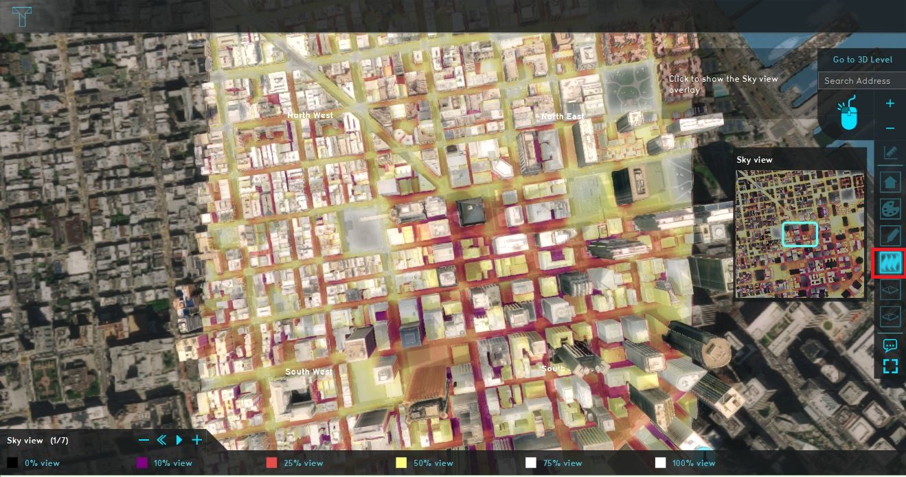
| | # Now click on the [[Sky_view_result_type_(Heat_Overlay)|Sky View overlay]]. This overlay shows the amount of sky visible from the street in direct line of sight (not hindered by any objects). Due to the high rise buildings, the sky view from some of the streets is minimal. To read more about how the sky view is calculated, see the used [[Sky_view_factor_calculation_model_(Heat_Overlay)|calculation method]]. |
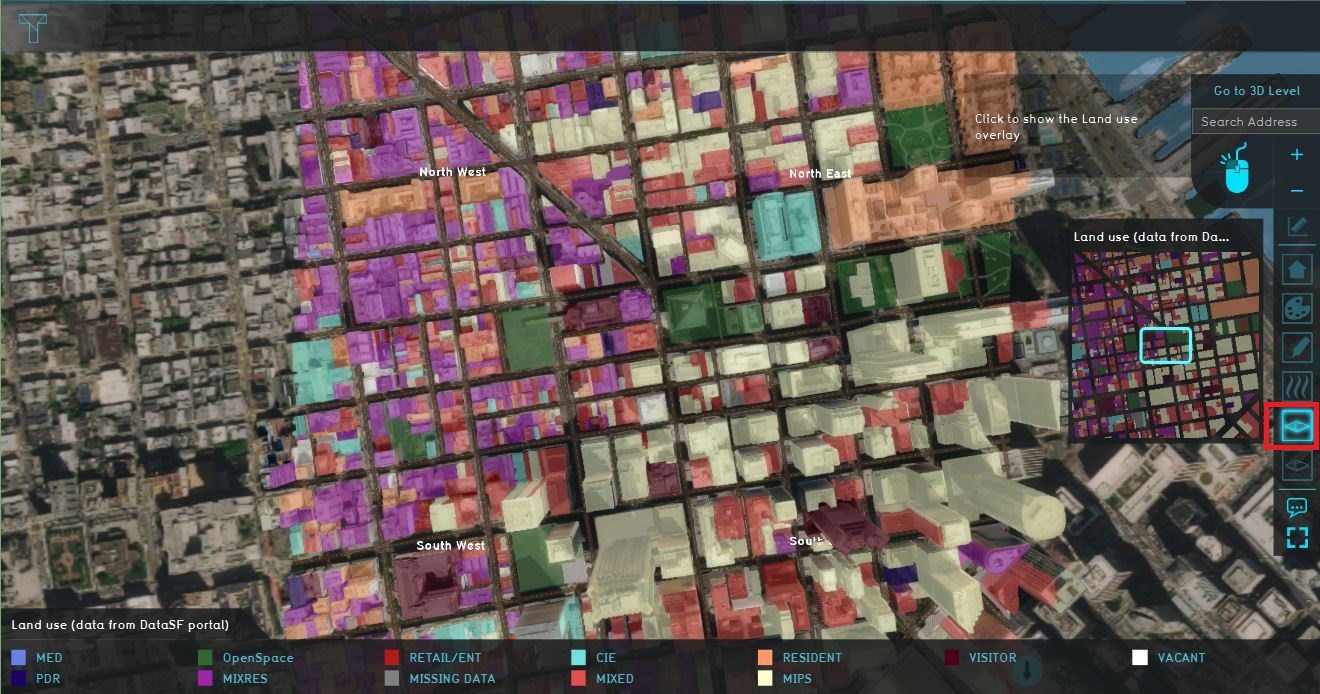
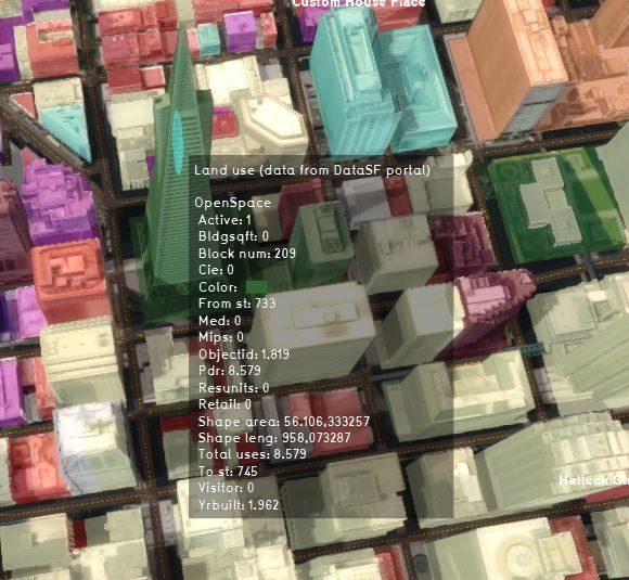
| | # The next overlay is the Land use map. This overlay shows the Land use dataset downloaded and imported from [https://data.sfgov.org/Housing-and-Buildings/Land-Use/us3s-fp9q the DataSF website]. Click on some buildings to see more information (attributes) about a particular building or area. |
|
| |
|
| [[File:Kockengen_figure01.PNG|800px]] | | [[File:Sources_i3s.JPG|right|150px|Notice that the I3S dataset is checked. The Data Sources Overview shows where the I3S data is used.]] |
|
| |
|
| ==Adding a Rainfall Overlay==
| | :''Proceed to the next page for more information and to read how to create a video or screenshot.'' |
| Follow these steps below to add a Rainfall Overlay:
| |
| # Hover over the button ''Overlays'', in the ''current situation tab'' and select Add Rainfall. The rainfall overlay is added to the Overlays in the left-side-panel. And in the overlay bar on the right side of the map.
| |
| # Select the Rainfall overlay in the left side panel and take a moment to familiarize yourself with the tabs in the right panel: General, Keys, Legend and Attributes
| |
| #* General contains the most common information necessary to interpret the rainfall overlay.
| |
| #* In Keys you can relate settings for the Rainfall overlay to attribute information stored in the 3D world.
| |
| #* Legend allows you to customize your legend
| |
| #* Attributes contains the general settings of the Rainfall overlay.
| |
| # Click on the ''Configuration Wizard'' button (see image below).
| |
| [[File:Kockengen_figure02.PNG|800px]]
| |
| | |
| With the Rainfall Wizard, you can configure your water system, this includes:
| |
| * The setup of the weather boundary condition
| |
| * Definition of the water system, including water level areas (peilgebieden), sewer districts and hydrological structures
| |
| * Setting of hydrological parameters
| |
| | |
| ==The Rainfall Wizard==
| |
| | |
| [[File:Kockengen_figure03.PNG|500px]]
| |
| | |
| With the Rainfall Overlay Wizard you can configure your water system. In this part of the tutorial we are going to use the following [[GeoJSON|GeoJSON-files]] (which you have downloaded at the start of this tutorial):
| |
| * waterlevelareas.geojson
| |
| * sewerdistricts.geojson
| |
| * weirs.geojson
| |
| * overflow.geojson
| |
| Some [[Import_Geo_data#Requirements|tips for using vector data files]] for the [[Water_Overlay]]:
| |
| * All files need to have a coordinate reference system (CRS) defined, for the {{software}} to place the data on the correct location.
| |
| * Hydraulic structures (weirs, culverts, pumps and overflows) should be imported as polygons, but translated in the {{software}} to either work as point- or line based structures. Read [[Hydraulic_structures_(Water_Overlay)#Types|here]] more about this difference.
| |
| | |
| [[File:Kockengen_figure04.PNG|600px]]
| |
| | |
| ===Step 1: defining the weather===
| |
| Press Next to proceed to the Weather panel, here the user can define rainfall and evaporation input, simulation time, which area of the project to calculate and the groundwater mode. Select the Option 'Linear' for rainfall over time. Change all numbers according to this picture:
| |
| | |
| [[File:Rainfall_wizard_step1.JPG|500px]]
| |
| | |
| With this settings you have defined a rainfall event:
| |
| * Uniform rainfall in 120 minutes
| |
| * With a total rainfall amount of 50mm
| |
| * With a dry period after rainfall of 120 minutes, so a total simulation time of 4 hours
| |
| * The whole project area will be (re)calculated.
| |
| * Reference evapotranspiration will be assumed on 1.5mm/day
| |
| * For groundwater, we assume that there is only infiltration. Read the information on the [[Ground water (Water_Overlay)|Groundwater mode]] to understand what this means for the calculation.
| |
| | |
| ===Step 2: setup of the water system===
| |
| Press next to proceed to the introduction screen: Setup Water System. In the following steps we will set up the water system using the prepared GeoJSONS. [[File:Kockengen_figure05B.PNG|thumb|250px|right]]
| |
| | |
| ====Step 2.1: adding water level areas====
| |
| Press next to the screen for importing water areas. A [[Water_level_area_(Water_Overlay)|water level area]] is an area with a spatially uniform water level varying in time. Variation can be caused by rainfall, evaporation on the surface water, inflow from sewer areas and inflow from the surface.
| |
| [[File:Kockengen_figure06.PNG|thumb|250px|right]] [[File:Kockengen_tutorial_waterlevel_areas.JPG|thumb|250px|right]]
| |
| There are several options to define your water level areas:
| |
| * Do Nothing: no water levels are used. Water terrains will be dry
| |
| * Import Water Areas: allows you to import a set of water level areas
| |
| * Generate Water Areas: allows you to define 1 water level area for your project area with 1 water level
| |
| * Select existing water level areas based on attribute: allows you to connect already imported water level data by using an existing attribute of this dataset
| |
| | |
| Select Import Water Level Areas (start Geo data wizard) and press Import Water Level Areas. The [[Geo_Data_Wizard|Geo Data Wizard]] will open. We will import waterlevelareas.geojson. Use the following attributes in the GeoJSON file as attributes for the Rainfall Overlay:
| |
| * WATERLEVEL: the [[Water_level_(Water_Overlay)|initial Water Level]] in the water level area (m + datum)
| |
| * NAME: the name of the water level area
| |
| | |
| Steps in the Geo Data Wizard:
| |
| # Select Import a GeoJSON file and press Next. Press Select File and locate the waterlevelareas.geojson. Press Open and press Next.
| |
| # An overview of your areas is generated; see right-side pictures. Press Next
| |
| # In the next step you can filter features based on an existing attribute. We skip this step (because we do not want the filter our dataset) by pressing Next
| |
| # We assign names to the water level areas using the NAME attribute from the geojson; see right-side pictures. Press Next
| |
| # We select all attributes, importing all attribute data from the geojson, and press Next. Note that only numerical attributes can be imported in to the {{software}}.
| |
| # We assign the WATERLEVEL attribute of the GeoJSON to the WATER_LEVEL key of the overlay; see right-side pictures
| |
| # At Finalize we press Finish to upload the areas to the server
| |
| | |
| After importing your water level areas you can review all parameters by opening the selection menu. Take some time to review the attribute values. What is the meaning?
| |
| | |
| ====Step 2.2: initial groundwater level====
| |
| In step 2.2, you can specify ground water levels. Since this tutorial is about Rainfall, we choose the default option ('Do Nothing')[[File:Kockengen_tutorial_groundwater.JPG|thumb|250px|right]]; see right-side picture.
| |
| | |
| ====Step 2.3: adding sewer areas====
| |
| [[Sewer_area_(Water_Overlay)|Sewer districts]] are represented by areas which have one [[Sewer_storage_(Water_Overlay)|storage value [m]]], uniform in space. Sewer storage will vary in time by sewer inflow from [[Sewered_(Water_Overlay)|connected buildings (buildings, roads, etc)]], pumped outflow to a WWTP (in the {{software}} this is to an external area outside of the project) and [[Sewer_overflow_(Water_Overlay)|sewer overflow]] to surface water.
| |
| In the wizard there are several options for defining the sewer system:
| |
| * Do nothing: no sewer areas are defined, this means that there is no sewerage in the project
| |
| * Import sewers: import sewer data
| |
| * Generate sewers: let the {{software}} [[How_to_generate_a_sewer|generate sewer areas]], based on adjustable parameters
| |
| * Select existing sewers based on attribute: if you already have sewer areas imported, you can connect them by selecting the attributes of the data to the overlay keys
| |
| | |
| Press import sewers and import the file sewerareas.geojson via the Geo data wizard. Assign the following attributes:
| |
| * NAME: name of the sewer district
| |
| * POC: [[Sewer_pump_speed_(Water_Overlay)|pump capacity assigned to the sewer district [m3/s]]]
| |
| * STORAGE: [[Sewer_storage_(Water_Overlay)|storage of the sewer district [mm]]] [[File:Kockengen_tutorial_sewer_attributes.JPG|thumb|250px|right]]
| |
| Follow the steps in the Geo Wizard according to the steps described in the water level areas section:
| |
| * At step 5, multiply the attribute value for STORAGE in the GeoJSON (mm) by 0,001 (conversion to m); see right-side pictures.
| |
| * At step 6, assign the the STORAGE attribute to the SEWER_STORAGE key and the POC attribute to the SEWER_PUMP_SPEED key
| |
| | |
| Take some time to review the attribute values in the imported area Kockengen. What is the meaning?
| |
| For more information on the sewer model, read the [[Sewer_model_(Water_Overlay)|Wiki]] page.
| |
| | |
| ====Step 2.4: adding inundation areas====
| |
| [[Inundation_area_(Water_Overlay)|Inundation areas]] are used to represent inundated or flooded areas in advance of the model's simulation. The following options are available:
| |
| * Do Nothing: there is no inundation area
| |
| * Import Water Areas: allows you to import inundation area(s) from an own dataset
| |
| * Generate Water Areas: allows you to define 1 inundation area with one water level for your whole project area
| |
| * Select existing water level areas based on attribute: allows you to connect already imported inundation data by using the water level attribute of this dataset
| |
| | |
| In this Tutorial, choose the default option (''Do Nothing)''.
| |
| | |
| ====Step 2.5: adding hydraulic structures====
| |
| In the [[Water_Overlay_Wizard|configuration wizard]] it is possible to import the following hydraulic structures:
| |
| * [[Weir_(Water_Overlay)|Weirs]]
| |
| * [[Culvert_(Water_Overlay)|Culverts]]
| |
| * [[Pump_(Water_Overlay)|Pumps]]
| |
| * [[Inlet_(Water_Overlay)|Inlets]]
| |
| * [[Sewer_overflow_(Water_Overlay)|Sewer overflows]]
| |
| | |
| ====2.5.1 adding weirs====
| |
| You can upload weirs.geojson by selecting Import Weirs in the Weirs screen and pressing Import Weirs. We will import weirs.geojson, using the following attributes:[[File:Kockengen_figure10.PNG|thumb|250px|right]]
| |
| * NAME: the name of the weir
| |
| * WEIR_HEIGHT: the [[Weir_height_(Water_Overlay)|crest height [m + datum]]]; to be assigned to the WEIR_HEIGHT key
| |
| * WEIR_WIDTH: the [[Weir_width_(Water_Overlay)|width of the crest [m]]]; to be assigned to the WEIR_WIDTH key
| |
| * WEIR_COEFF: tthe [[Weir_coefficient_(Water_Overlay)|flow coefficient related to the shape of the weir]]; to be assigned to the WEIR_COEFFICIENT key
| |
| | |
| In the Geo Wizard follow the steps:
| |
| # Select Import a GeoJSON file and press Next. Press Select File and locate the wiers.geojson. Press Open and press Next.
| |
| # An overview of your areas is generated as below. Press Next
| |
| # In the next step you can filter features based on attribute filtering. We skip this step by pressing Next
| |
| # We assign names to the water level areas using the NAME attribute from the GeoJSON and press Next
| |
| # We select all attributes, importing all attribute data from the GeoJSON, and press Next
| |
| # We assign the WEIR_HEIGHT attribute of the GeoJSON to the WEIR_HEIGHT key of the overlay, the WEIR_WIDTH attribute of the GeoJSON to the WEIR_WIDTH key of the rainfall overlay and the WEIR_COEFF attribute of the GeoJSON to the WEIR_COEFFICIENT attribute of the rainfall overlay. [[File:Rainfall_weirs_keys.JPG|thumb|250px|right]]
| |
| # At Finalize we press Finish to upload the areas to the server
| |
| | |
| Take some time to review the attribute values. What is the meaning? <br>
| |
| Notice that there is also a weir angle attribute, read the [[Weir_angle_(Water_Overlay)|wiki]] to know what this attribute is used for.
| |
| <br>
| |
| <br>
| |
| [[File:Rainfall_weirs_updated.JPG|500px]]
| |
| | |
| ====2.5.2 adding culverts====
| |
| Click next to proceed to the step for importing culverts. Notice that there are already culverts imported. On the [[Project_Sources|project sources]] page you can read where this data comes from (last entry in the table). Select some culverts from the drop down menu and click on Show in Editor to see where they are located in the 3D world. Since from the open dataset not all attributes are known, for example the [[Culvert_diameter_(Water_Overlay)|culvert diameter]] is by default set to 1m. Notice that there are some errors. These culverts are marked red in the drop down menu and also the step itself is marked red. Read some of the error messages given when selecting a marked red culvert in the drop down menu and proceed with the next step.
| |
| | |
| [[File:Culverts.JPG|500px]]
| |
| | |
| ====2.5.3 adding pumps & 2.5.4 adding inlets====
| |
| Similar to the import procedure of weirs, you can add pumps and inlets. In this tutorial, choose the default (''Do Nothing'').
| |
| | |
| ====2.5.5 Adding Overflows====
| |
| In this step we will add the [[Sewer_overflow_(Water_Overlay)|sewer overflow]]. Upload the overflows.geojson by selecting Import Overflows in the Wizard. We will import overflow.geojson, using the following attributes:
| |
| * LEVEL: the [[Sewer_overflow_attribute_(Water_Overlay)|crest level of the overflow]]; assign to the SEWER_OVERFLOW overlay key
| |
| * CAPACITY: the [[Sewer_overflow_speed_(Water_Overlay)|overflow capacity of the overflow]]; assign to the SEWER_OVERFLOW_SPEED overlay key
| |
| Follow the Geo Data Wizard similar to the procedure at importing weirs (see 2.5.1 adding weirs) and view the result. What do the values mean?
| |
| | |
| [[File:Kockengen_figure13.PNG|500px]]
| |
| | |
| ===Step 3: setup of coefficients===
| |
| In this step you can adjust default parameters related to the [[Surface_model_(Water_Overlay)|surface]] (e.g. roughness), [[Underground_model_(Water_Overlay)|sub-surface]] (e.g. conductivity) and infrastructure (e.g. is a type connected to a sewer or not). As we work with a 3D world containing a lot of data, the determination of model-coefficients can be complex. E.g.:
| |
| * A [[Water_manning_(Water_Overlay)|manning roughness coefficient]] can be related to the surface type (e.g. clay) if no infrastructure present. If infrastructure is present (e.g. a road), the value of the road will be used, and the value of the surface type will be ignored
| |
| * An [[Terrain_ground_infiltration_md_(Water_Overlay)|infiltration]] parameter can be related to the surface (land cover), [[Ground_infiltration_per_day_(Function_Value)|infrastructure]] or underground (sub-surface).
| |
| You can inspect each of the parameters by hovering or clicking on the question mark icon next to the parameter. We will leave everything to default by pressing next (4x)
| |
| <br>
| |
| <br>
| |
| [[File:Kockengen_figure14.PNG|500px]]
| |
| | |
| ===Step 4: Interactions===
| |
| Here you can choose to visualize your water system network in the rainfall overlay:
| |
| * Display Water System network: shows schematically the network of the water system
| |
| * Display Weirs with Panels: shows on the location of weirs a panel, allowing the user to overwrite structure settings
| |
| * Display Water level Areas with Panels: shows on all centroids of water level areas panels, allowing the user to overwrite initial water levels
| |
| | |
| [[File:Kockengen_figure15.PNG|500px]]
| |
| | |
| ===Step 5: Output Overlays===
| |
| Each water overlay can produce one or more results. By default the [[Waterstress_result_type_(Water_Overlay)|water stress]] is chosen, which is the amount of water on the surface. For water terrains a maximum allowed increase model parameter is set. Below that depth no water stress will be perceived. To see only the amount of water on the surface, select the [[Surface_last_value_result_type_(Water_Overlay)|surface last value]] and check the First checkbox, the [[Surface_elevation_result_type_(Water_Overlay)|surface elevation]] and the [[Base_types_result_type_(Water_Overlay)|base types]]. Read the wiki pages to understand what each result type will show. Also, unselect the water stress result type. Notice the number of [[Timeframes_(Water_Overlay)|Timeframes]] can be selected with the slider. The more timeframes, the more intermediate steps there are recorded and viewable for the user. Note that timeframes are not the same as [[Timestep_formula_(Water_Overlay)|timesteps]].
| |
| <br>
| |
| [[File:Rainfall_results.JPG|500px]]
| |
| | |
| ===Step 6: Input Overlays===
| |
| The Rainfall Overlay uses several input parameters to compute output. These input overlays can be visualized in the Input Overlays section. Select the [[Water_manning_(Water_Overlay)|manning roughness value [m/s^1/3]]].
| |
| | |
| [[File:Kockengen_figure17.PNG|500px]]
| |
| | |
| ===Step 7: Advanced Settings===
| |
| Here you can change some [[Model_attributes_(Water_Overlay)|model attributes]] for the [[Rainfall_(Overlay)|rainfall overlay]].
| |
| The attributes you can change in this step are:
| |
| * [[Max_water_depth_m_(Water_Overlay)| Max water depth attribute]]
| |
| * [[Max_water_bottom_m_(Water_Overlay)| Max water bottom attribute]]
| |
| * [[ Object_correction_(Water_Overlay)| Object correction attribute]]
| |
| * [[Shoreline_(Water_Overlay)| Shoreline attribute]]
| |
| Read the above Wiki pages, but keep the default values.
| |
| | |
| [[File:Advanced_settings_rainfall.JPG|500px]]
| |
| | |
| Press Finish to finalize the wizard
| |
| | |
| ==After completion of the wizard==
| |
| [[File:Kockengen_tutorial_general_tab.JPG|thumb|150px|right|The general tab in the right panel]]
| |
| [[File:Kockengen_tutorial_inactive_copyJPG.JPG|thumb|150px|right|The inactive copy of the Rainfall overlay is greyed out]]
| |
| After finishing the wizard, you need to [[Grid_Overlay#Grid_recalculation|Update the grid]] to recalculate the rainfall overlay. Every time you change a parameter in the model, whether that is in the wizard or in the editor itself, the overlay has to be recalculated by pressing Update Now. However, if the [[Calculation_panel#Auto-update_indicators|auto update]] is on, the overlay is automatically recalculated when changing a parameter in the wizard. When working in/with a large project, a small grid size, long simulation time etc., it can be desirable to turn the auto update off in order to not have to wait every time on the recalculation of the overlay, until you are done with editing and ready for the results. When dealing with very long calculations, take note of the [[Peak_hours|peak hours]], the option to [[Calculation_panel#GPU_overview|cancel]] the calculation (if you notice that it will take a long time) and the option to [[Grid_Overlay#Delayed_calculation|delay]] the calculation.
| |
| | |
| When the calculation is finished, please explore the following interesting features:
| |
| <br>
| |
| [[File:Results_kockengen.JPG|500px]]
| |
| <br>
| |
| * Play the overlay by clicking on the arrows in the bottom left corner of the 3D world. Can you explain what happens?
| |
| * Click in the left panel on the other overlays. Can you explain the results? Notice the [[Base_types_result_type_(Water_Overlay)|base types]] result. This result type shows input used for the model. As you can see the division in land, water and constructions is very rough. This is related to the [[grid cell size]]. In the General Tab you can press ''Change Grid'' to change the [[grid cell size]] to for example 2m. Can you see the difference, and see the impact on the [[Surface_last_value_result_type_(Water_Overlay)|surface last value]], timesteps and calculation time?
| |
| * Open the Rainfall Wizard again and click on the culverts step. Notice there are less errors with the culverts by changing the grid cell size. Can you now follow the error messages that were previously given?
| |
| * In the General Tab you can show the [[Results (Water Overlay)#Water balance|Water Balance]]. Please explore.
| |
| * Below there is a summary, the [[Results (Water Overlay)#Debug info|debug info]], please explore.
| |
| * In the General Tab, you can specify the [[Calculation_preference_formula_(Water_Overlay)|Calculation Preferences]].
| |
| * In the General Tab you can [[Geo_Data#Export_raster_data|export the result]] as a [[GeoTiff]]. Please do so and visualize your result in a GIS, for example QGIS.
| |
| * In the General Tab, click on ''Save overlay result''. Notice what happens: an inactive copy of the result type is created in the overlay left panel. This [[Results (Water Overlay)#Storing_specific_overlay_result|inactive copy]] can be used to store results, from for example a specific rain event, and compare it later with another result type of another rain event.
| |
| * In the General Tab, [[Warning and recommendations (Water Overlay)|warnings]] may also appear, for example about the accuracy of the model in relation to the grid cell size.
| |
| * Create an overlay of the water level areas to provide more insight. Follow the (general) steps [[Geo_Data_tutorial#Create_an_overlay|in the Geo Data tutorial]] for creating an overlay of the already imported water level areas.
| |
| * Open the Rainfall Wizard again. Select more and/or different result types and update the Rainfall overlay. Can you display and interpret the results?
| |
| | |
| ===Extra step: measuring tool===
| |
| The {{software}} also provides a measurement tool to create sections. Read [[Measuring_tool|here]] more about this measuring tool.
| |
| Try to create a line measurement with the same settings as below in the image. Make sure the result type that you are displaying is the [[Surface_last_value_result_type_(Water_Overlay)|surface last value]]. Can you explain what you see in the graph?
| |
| <br>
| |
| [[File:Measurement_tutorial.JPG|500px]]
| |
| <br> | | <br> |
| The created section shows the amount of water on the surface (m + datum) in yellow and the terrain height in red. When you play the overlay, you will see the yellow line moving according to the amount of water that is on the surface during that timeframe. Make some more measurements on different places. | | <gallery> |
| | File:Sources_i3s.JPG|2. Notice that the I3S dataset is checked. The Data Sources Overview shows where the I3S data is used. |
| | File:City_overlay.JPG|4. Click on the City overlay to go to the default view. |
| | File:Select_building_project.JPG|5. Click in the Current tab on the Buildings button and click on the building with the arrow. |
| | File:Attributes_building.JPG|5. The attributes of the building. |
| | File:Building_details.JPG| 6. Click on the Details tab to see the Function values. |
| | File:Hotel_data.JPG|7. Click on the pen icon. A map with the hotels in the project is now visualized. |
| | File:Hotel_more_information.JPG|8. Click on one of the purple buildings and notice the information in the hover panel. |
| | File:Sky_view_data.JPG|9. Click on the Sky view map. |
| | File:Land_use_data.JPG|10. Click on the Land use map. |
| | File:Land_use_more_info.JPG| 10. Click on one of the buildings to see more information in the hover panel. |
| | </gallery> |
|
| |
|
| You have now finished the tutorial!
| | {|class="wikitable" style="margin: auto; background-color:#ffffcc;" |
| {{Water Module buttons}}
| | | [[Demo_San_Francisco_Project_FAQ_%26_More|Next page>>]] |
| | |} |


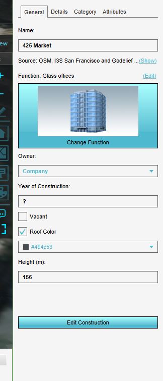 We are going to inspect one of the buildings in the model. Therefore click on the Current situation tab on the Buildings button and select the building that is referred to with the arrow icon. In the right panel, the attributes such as the name of the building and its function are displayed. Notice that this building has the function office, which is known from the OSM dataset.