Flooding Overlay

What is the Inundation overlay

The inundation is developed for the computation of surface (water) flow in a wide range of applications. These applications include large scale inundations due to dike breaches and inundations at the bottom of hill-slopes. Therefore the commonly applied 2D Saint Venant Equations are implemented on a highly parallel applicable explicit numerical scheme suitable for Tygron GPU clusters.

Adding and removing

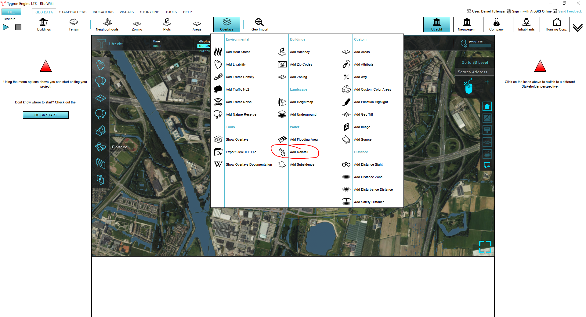
To add an inundation overlay go to the Overlays menu in the GEO DATA ribbon and select Add Inundation. To remove the overlay, press Remove below the overlays list.

Result types

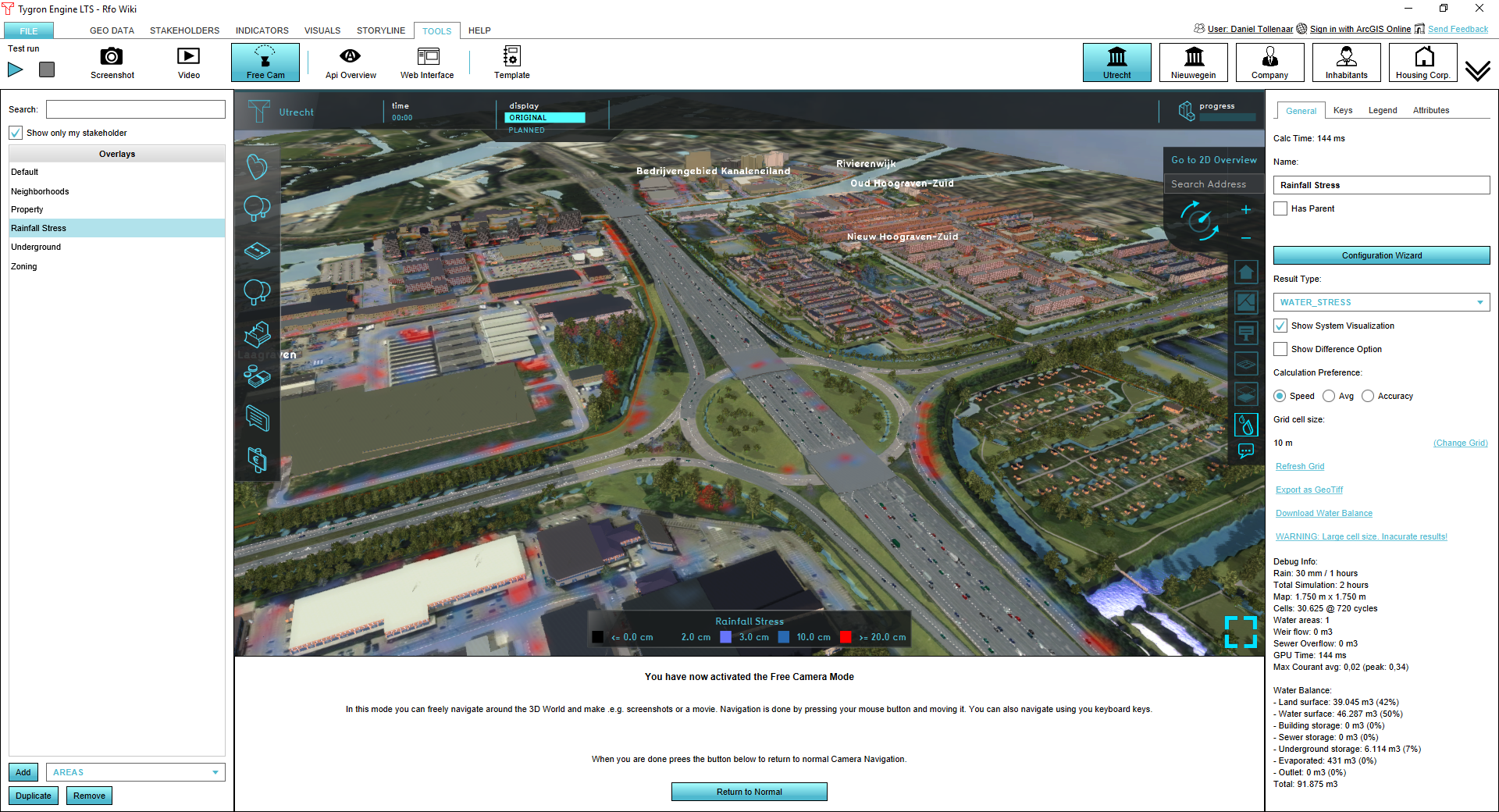
The rainfall overlay is a grid overlay showing results of heavy rainfall on the surface (flooding), sub-surface (groundwater), open water and sewer system. The following results are produced:

Result type	Unit	Description
BASE_GROUNDWATER_DISTANCE	m (below surface)	Initial groundwater level relative to the surface level (NL: ontwateringsdiepte).
BASE_TYPES	nominal value	Division of gridcells in water, land or sewer areas that are connected to the sewer.
EVAPORATED	m (mm)¹	Total evaporation over the simulation period
IMPACTED_BUILDINGS	nominal value	Constructions impacted by flood: the value from the function value indicator is assigned to a building if the water depth at a grid-cell surrounding the building exceeds the overlay attribute value IMPACT_FLOOD_TRESHOLD_M
SEWER_LAST_VALUE	m (mm)¹	The amount of water in the sewer storage at the end of simulation
SEWER_MAX_VALUE	m (mm)¹	Maximum amount of water in the sewer storage during the simulation
SURFACE_DURATION	s (min)¹	The amount of time the water depth in a cell exceeds the value set in the overlay attribute value SHOW_DURATION_FLOOD_LEVEL_M
SURFACE_FLOW	m3/m2	Total volume of water passed a grid-cell, scaled by the cell surface (grid cell-size^2)
SURFACE_LAST_VALUE	m (min)¹	Water depth at the end of simulation
SURFACE_MAX_VALUE	m (min)¹	Maximum water depth during the simulation
UNDERGROUND_FLOW	m³/m²	Totall infiltration amount from the surface to groundwater
UNDERGROUND_LAST_VALUE	m (mm)	The amount by which the groundwater table has risen above the initial groundwater level at the end of simulation
UNDERGROUND_MAX_VALUE	m (mm)	The maximum amount by which the groundwater table has risen above the initial groundwater during the simulation
WATER_STRESS	m (mm)	The Maximum water depth during the simulation. At water cells only a water depth is shown if the depth exceeds the overlay attribute value ALLOWED_WATER_INCREASE_M

¹ the units between () are as displayed in the 3D client. If exported to GTiff the SI-convention is used: meters (m) and seconds (s).

Inundation Model

2D Saint Venant equations

The 2D Saint Venant equations describe the conservation of mass in a gridcell and the conservation of momentum in both x and y, direction:

The Saint Venant equations describe the following processes:

• friction
• bed slope
• water pressure
• convection (changes in bathemetry over space)
• inertia (increase or decrease of velocity over time)

Numerical scheme

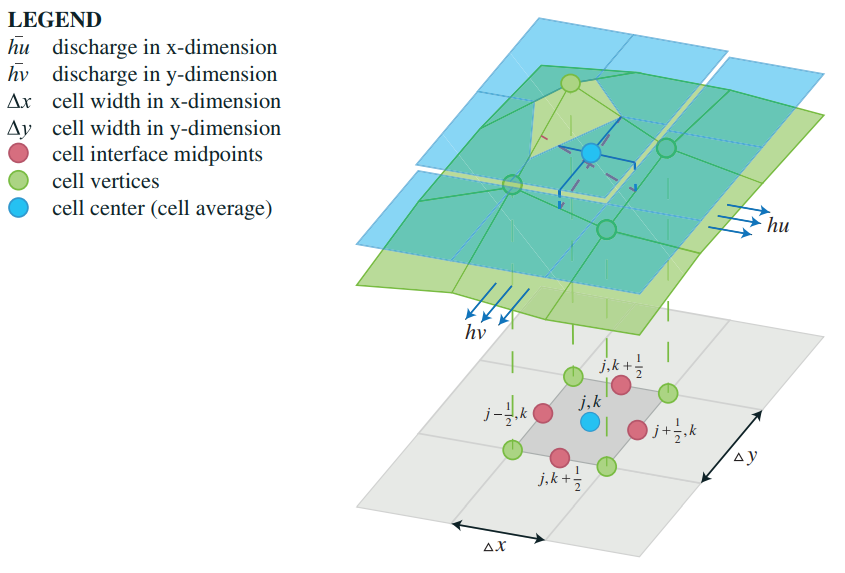
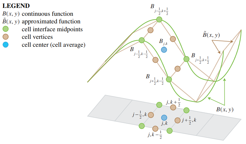
The explicit second-order semi-discrete central-upwind scheme for the 2D Saint Venant Equations is implemented. A reconstruction of cell bottom, water level and velocity at the interfaces between computational cells as proposed by Lax and Wendroff (Rezzolla, 2011). The Tygron Engine Inundation module relies on the scheme described in Kurganov and Petrova (2007). The reconstruction method is taken from Bolderman et all (2014) and ensures numerical stability at the wetting and drying front of a flood wave.

1. The elevation value of the cell is equal to the elevation value at the centre of the cell. At the same time, it is equal to the average value of the elevation values at the cell interface mitpoints
2. The slopes of the conserved variables, continuity and momentum in x and y direction, are reconstructed
3. Values at the cell interface midpoints are compared with the left-sided and right sided values at cell centres
4. At partially dry cells, the slope is modified to both avoid negative depths and numerical instability
5. (Numerical) fluxes are computed at each cell interface to determine the conserved variable of the next time-step

The numerical scheme as been tested on the benchmark of the UK Environmental Agency

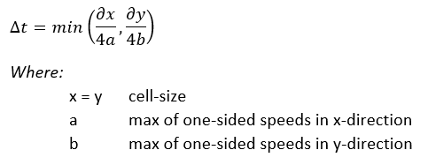
Computation time step

An adaptive timestep is implemented according to Kurganov and Petrova (2007). At every timestep, the courant-number is kept smaller than 0.25 for every active computation cell:

References

1. Bollermann A, Chen G, Kurganov A and Noelle S (2014) ∙ A Well-Balanced Reconstruction For Wetting/Drying Fronts ∙ found at: https://www.researchgate.net/publication/269417532_A_Well-balanced_Reconstruction_for_Wetting_Drying_Fronts (last visited 2018-06-29)
2. Environmetal Agency (2013). Benchmarking the latest generation of 2D hydraulic modelling packages ∙ report Report – SC120002 ∙ found at: https://consult.environment-agency.gov.uk/engagement/bostonbarriertwao/results/appendix-6---neelz--s.---pender--g.--2013--benchmarking-the-latest-generation-of-2d-hydraulic-modelling-packages.-bristol_environment-agency.pdf (last visited 2018-08-03)
3. Kurganov A, Petrova G (2007) ∙ A Second-Order Well-Balanced Positivy Preserving Central-Upwind Scheme for the Saint-Venant System ∙ found at: http://www.math.tamu.edu/~gpetrova/KPSV.pdf (last visited 2018-06-29)
4. Rezzolla L (2011) ∙ Numerical Methods for the Solution of Partial Differential Equations ∙ found at: http://www.scirp.org/(S(lz5mqp453edsnp55rrgjct55))/reference/ReferencesPapers.aspx?ReferenceID=1886006 (last visited 2018-06-29)
5. Zsolt Horváth1, Jürgen Waser, Rui A. P. Perdigão, Artem Konev and Günter Blöschl (2014) ∙ A two-dimensional numerical scheme of dry/wet fronts for the Saint-Venant system of shallow water equations ∙ found at: http://citeseerx.ist.psu.edu/viewdoc/download?doi=10.1.1.700.7977&rep=rep1&type=pdf ∙ http://visdom.at/media/pdf/publications/Poster.pdf ∙ (last visited 2018-06-29)