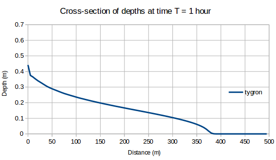
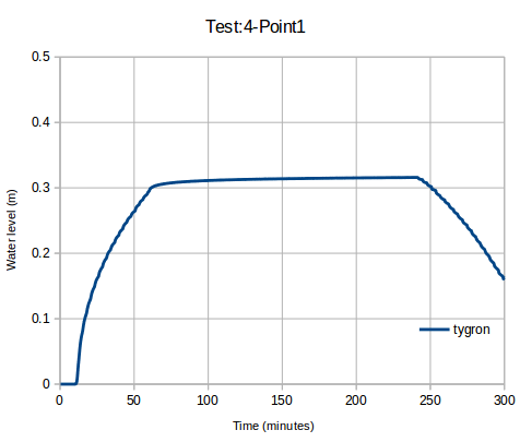
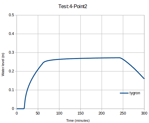
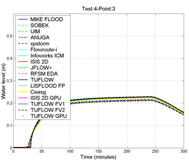
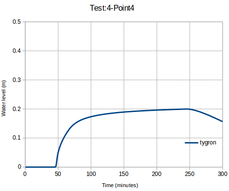
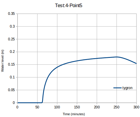
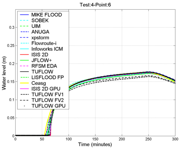
<li style="display:inline-block">[[File:crosssection_waterlevel_1h_case4_ukbm.png|thumb|left|x300px|Water level at t = 1 h.]]</li>
<li style="display:inline-block">[[File:crosssection_waterlevel_1h_case4_ukbm.png|thumb|left|x300px|Water level across center line at t = 1 h.]]</li>
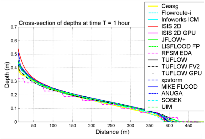
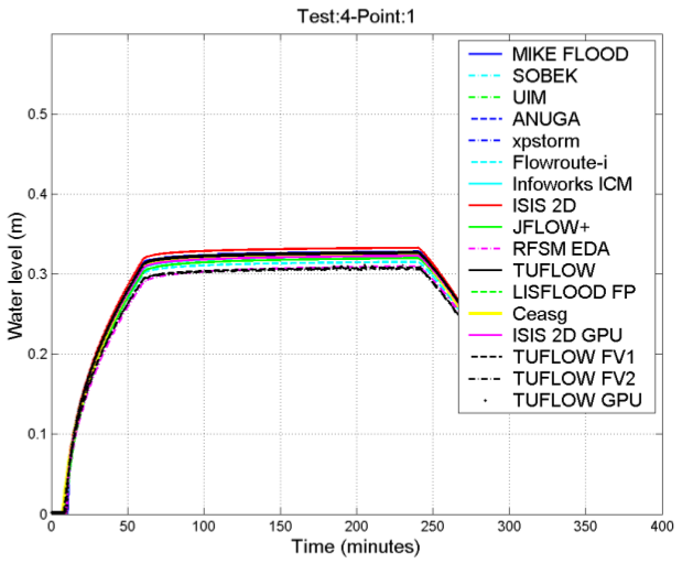
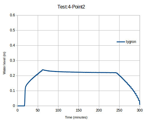
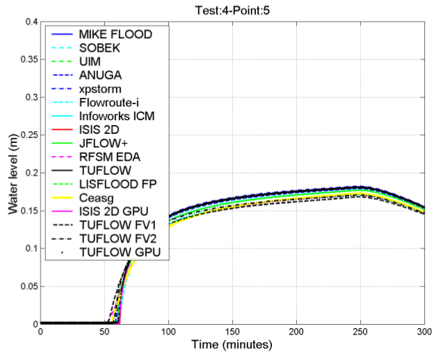
<li style="display:inline-block">[[File:crosssection_waterlevel_others_1h_case4_ukbm.png|thumb|left|x300px|Water level at t = 1 h for other packages.]]</li><br>
<li style="display:inline-block">[[File:crosssection_waterlevel_others_1h_case4_ukbm.png|thumb|left|x300px|Water level across center line at t = 1 h for other packages.]]</li><br>
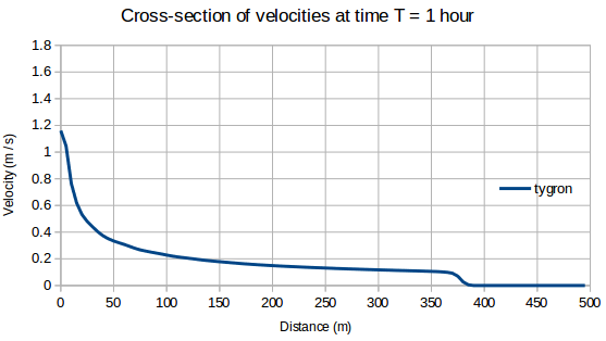
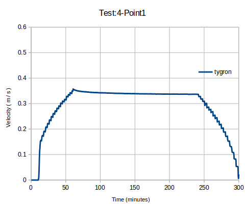
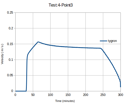
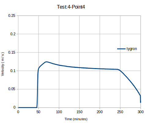
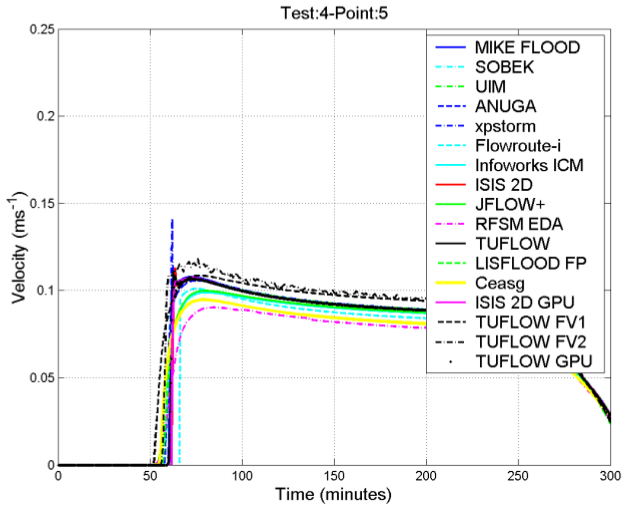
<li style="display:inline-block">[[File:crosssection_velocity_1h_case4_ukbm.png|thumb|left|x300px|Flow velocity at t = 1 h.]]</li>
<li style="display:inline-block">[[File:crosssection_velocity_1h_case4_ukbm.png|thumb|left|x300px|Flow velocity across center line at t = 1 h.]]</li>
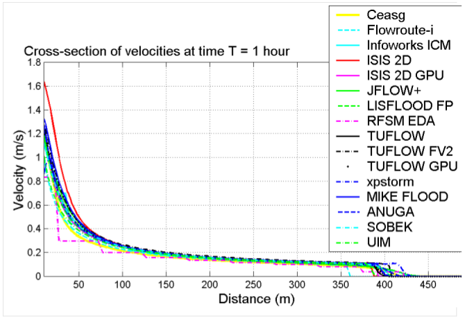
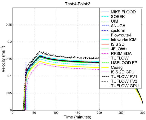
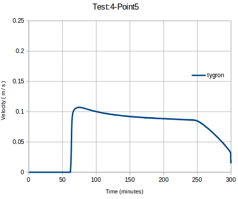
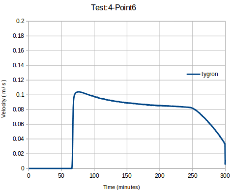
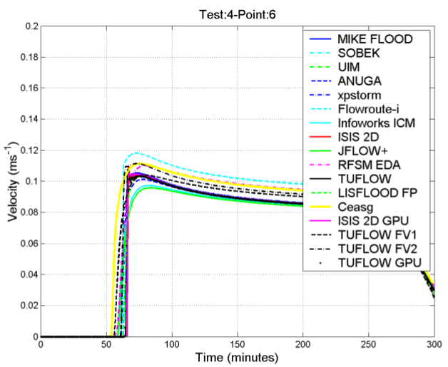
<li style="display:inline-block">[[File:crosssection_velocity_others_1h_case4_ukbm.png|thumb|left|x300px|Flow velocity at t = 1 h for other packages.]]</li>
<li style="display:inline-block">[[File:crosssection_velocity_others_1h_case4_ukbm.png|thumb|left|x300px|Flow velocity across center line at t = 1 h for other packages.]]</li>
</ul>
</ul>
Revision as of 14:49, 2 May 2019
This page reports on the performance of the Tygron Platform's Water Module by means of the UK EA Benchmark Test 4 – Speed of flood propagation over an extended floodplain.
The objective of this test is to assess the package’s ability to simulate the celerity of propagation of a flood wave and predict transient velocities and depths at the leading edge of the advancing flood front. It is relevant to fluvial and coastal inundation resulting from breached embankments.[1]
Description
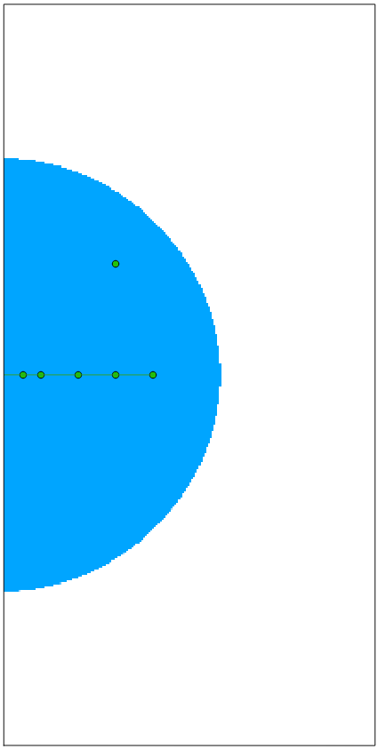
This test is designed to simulate the rate of flood wave propagation over a 1,000 x 2,000 m floodplain following a defence failure (Fig. (a)). The floodplain surface is horizontal, at datum (= 0 m). One inflow boundary condition will be used, simulating the failure of an embankment by breaching or overtopping, with a peak flow of 20 m3/s and time base of ~6 h. The boundary condition is applied along a 20-m line in the middle of the western side of the floodplain.[1]
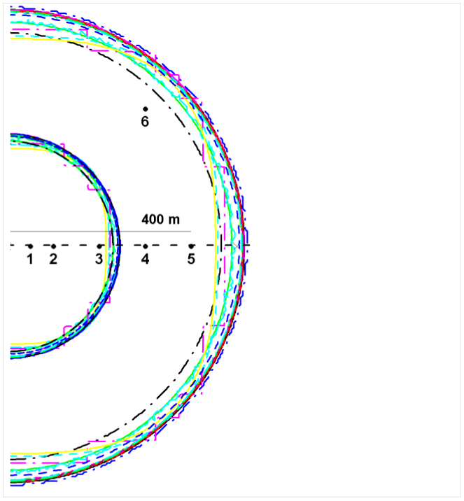
Figure (a): Modelled domain and the locations of the 20-m line of inflow, 6 output points, and the aimed for 0.1-m and 0.2-m contour lines at t = 1 h (dashed) and t = 3 h (solid), respectively.Animation of the test result for case 4, generated by the Tygron Platform. Map dimensions = 1,000 x 2,000 m. Grid-cell size = 5 m.Figure (b): Hydrograph applied as inflow boundary condition.
Boundary and initial condition
Inflow boundary condition as shown in Fig. (b)
All other boundaries are closed
Initial condition: dry bed
Parameter values
Manning’s n: 0.05 (uniform)
Model grid resolution (m): 5 (or ~80,000 nodes in the area modelled)
Simulated time (h): 5
Required output
Point ID
X
Y
1
50
1,000
2
100
1,000
3
200
1,000
4
300
1,000
5
300
1,000
6
300
1,300
Software package used: version and numerical scheme
Specification of hardware used to undertake the simulation: processor type and speed, RAM
Minimum recommended hardware specification for a simulation of this type
Time increment used, grid resolution (or number of nodes in area modelled) and total simulation time to specified time of end
Raster grids (or TIN) at the model resolution consisting of:
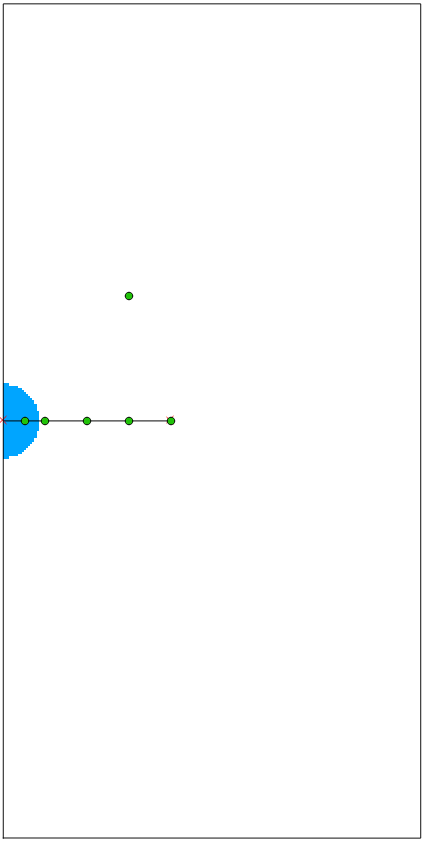
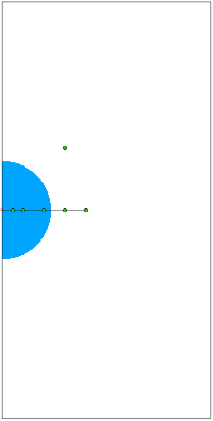
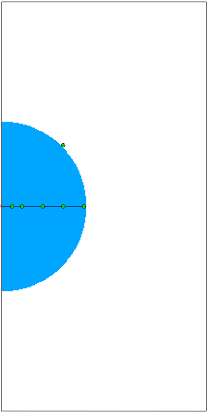
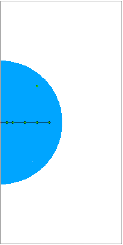
Depths and at t = 30 min, 1 h, 2 h, 3 h and 4 h
Velocities (scalar) at t = 30 min, 1 h, 2 h, 3 h and 4 h
Plots of velocity and water elevation v. time (suggested output frequency: 20 s) at the 6 locations represented in Fig. (a) and provided as part of dataset
Dataset content
Upstream boundary condition table (inflow v. time). Filename: Test4BC.csv
Location of output points. Filename: Test4Output.csv
The model geometry is as specified in Section 2. No DEM is provided, as the surface elevation is level at datum (= 0 m).[1]
Technical setup
Figure 1. The relative positions of the measurement points used in this test.
Flat surface
Grid-cell size (m): 5
Area size (m): 1,010 x 2,010 (required domain of 1,000 x 2,000 + 5-m border)
The measurement points were positioned correctly (see Fig. 1)
In order to regulate the boundary discharge according the hydrograph (Fig. 2), 2 inlets were implemented. Both inlets occupied one grid cell, one of these located above and the other below the green center line (Fig. 3). The inlets were configured as follows:
External area (m2): 1,000,000,000
Water level (m): 1
Threshold (m): none
Inlet Q (m):
Figure 2. Hydrograph displaying the implemented individual and combined inlet fluxes.
Figure 3. Positions of the inlet cells (red squares) with respect to the center line of measurement (green).


