Flooding Overlay

What is the Flooding overlay

The Flooding Overlay is developed for the computation of surface (water) flow in a wide range of applications. These applications include large scale inundations due to dike breaches and inundations at the bottom of hill-slopes. Therefore the commonly applied 2D Saint Venant Equations are implemented on a highly parallel applicable explicit numerical scheme suitable for Tygron GPU clusters.

Adding and removing

How to add the Flooding Overlay:

1. Select in the editor 'Geo Data' from the ribbon
2. Select 'Overlays' from the ribbon bar
3. Select the Flooding Overlay from the drop down menu

How to remove the Flooding Overlay:

1. Select in the editor 'Geo Data' from the ribbon
2. Select 'Overlays' from the ribbon bar
3. Select the Flooding Overlay from the list of active overlays on the left panel
4. Select 'remove' from the bottom of the left panel
5. Confirm the removal in the pop up confirmation message

Result types

The Flooding Overlay is a grid overlay showing results of a dike breach/heavy rainfall on the surface (flooding), sub-surface (groundwater), open water and sewer system. For the produced results, see the result types of the Rainfall Overlay.

Inundation Model

2D Saint Venant equations

The 2D Saint Venant equations describe the conservation of mass in a gridcell and the conservation of momentum in both x and y, direction:

The Saint Venant equations describe the following processes:

• friction
• bed slope
• water pressure
• convection (changes in bathemetry over space)
• inertia (increase or decrease of velocity over time)

Numerical scheme

The explicit second-order semi-discrete central-upwind scheme for the 2D Saint Venant Equations is implemented. A reconstruction of cell bottom, water level and velocity at the interfaces between computational cells as proposed by Lax and Wendroff (Rezzolla, 2011). The Tygron Platform Inundation module relies on the scheme described in Kurganov and Petrova (2007). The reconstruction method is taken from Bolderman et all (2014) and ensures numerical stability at the wetting and drying front of a flood wave.

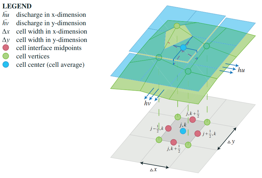
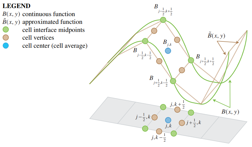
A clear explanation on the numerical approach can be found at Horváth et al. (2014), but in general it follows these steps:

1. The elevation value of the cell (B in figures below) is equal to the elevation value at the center of the cell. At the same time, it is equal to the average value of the elevation values at the cell interface midpoints
2. The slopes of the conserved variables (U in figures below), continuity and momentum in x and y direction, are reconstructed
3. Values of conserved variables at the cell interface midpoints are compared with the left-sided and right sided values at cell centres
4. At partially dry cells, the slope is modified to both avoid negative depths and numerical instability
5. (Numerical) fluxes are computed at each cell interface to determine the values of the conserved variable at the cell centres for the next time-step

Source: Horváth et al. (2014)

The numerical scheme as been tested on the benchmark of the UK Environmental Agency (EA, 2013) and the Dutch STOWA (STOWA, 2017)

Computation time step

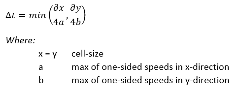
An adaptive timestep is implemented according to Kurganov and Petrova (2007). At every timestep, the courant-number is kept smaller than 0.25 for every active computation cell:

Especially at low depths, choosing the appropriate timestep is critical to avoid numerical instability. Therefore the following principles are used to determine the right time step:

• the timestep is choosen so that all computation cells follow one of the following criteria
• if a cells waterdepth is below the flooding threshold, 5 * 10&sup-3; (m) there is no flow assumed between that cell and it neigboring cell
• if the cells waterdepth is above above the flooding threshold, the maximum timestep is assumed to be 100 * the waterdepth at the cell
• if the waterdepth increases, the timestep is assumed to be not larger than the formula above

If he numerical flux decreases, the larger timesteps are allowed than set by Kurganov and Petrova, depending on the calculation preference set in the general tab of the inundation overlay (speed, average or accuracy).

References

1. Bollermann A, Chen G, Kurganov A and Noelle S (2014) ∙ A Well-Balanced Reconstruction For Wetting/Drying Fronts ∙ found at: https://www.researchgate.net/publication/269417532_A_Well-balanced_Reconstruction_for_Wetting_Drying_Fronts (last visited 2018-06-29)
2. Environmetal Agency (2013). Benchmarking the latest generation of 2D hydraulic modelling packages ∙ report Report – SC120002 ∙ found at: https://consult.environment-agency.gov.uk/engagement/bostonbarriertwao/results/appendix-6---neelz--s.---pender--g.--2013--benchmarking-the-latest-generation-of-2d-hydraulic-modelling-packages.-bristol_environment-agency.pdf (last visited 2018-08-03)
3. Kurganov A, Petrova G (2007) ∙ A Second-Order Well-Balanced Positivy Preserving Central-Upwind Scheme for the Saint-Venant System ∙ found at: http://www.math.tamu.edu/~gpetrova/KPSV.pdf (last visited 2018-06-29)
4. Rezzolla L (2011) ∙ Numerical Methods for the Solution of Partial Differential Equations ∙ found at: http://www.scirp.org/(S(lz5mqp453edsnp55rrgjct55))/reference/ReferencesPapers.aspx?ReferenceID=1886006 (last visited 2018-06-29)
5. STOWA (2017) ∙ Benchmark Inundatiemodellen, Modelfunctionaliteiten en testbankberekeningen ∙ found at: https://ruimtelijkeadaptatie.nl/publish/pages/129612/benchmark_inundatiemodellen_stowa_2017.pdf (last visited 2018-08-13)
6. Zsolt Horváth, Jürgen Waser, Rui A. P. Perdigão, Artem Konev and Günter Blöschl (2014) ∙ A two-dimensional numerical scheme of dry/wet fronts for the Saint-Venant system of shallow water equations ∙ found at: http://citeseerx.ist.psu.edu/viewdoc/download?doi=10.1.1.700.7977&rep=rep1&type=pdf ∙ http://visdom.at/media/pdf/publications/Poster.pdf ∙ (last visited 2018-06-29)